Every day, requests for information come into the applications departments of companies. Applications programmers are then asked to take the requests and use their expertise to retrieve that information from operational data. I am going to follow the path of one such request to illustrate a new tool available in Operations Navigator (OpsNav) for V4R5 that will help reduce the time spent optimizing the retrieval of information for that request.

The request for today is to produce a report of all the sales that resulted in a negative pre-tax profit. My marketing manager wants to review these reports on a weekly basis. I have just started using SQL statements to retrieve information from our tables, so I am going to try this as part of my solution to the problem.

Who Needs a Query Optimizer, Anyway?

Since I am new to writing SQL statements, I am not sure if I am writing the most efficient SQL statement to access the company’s data. I want to be very careful about running my queries on my production system, so how can I make sure this SQL is running reasonably? I have heard that DB2 for OS/400 includes a query optimizer, which helps to improve performance of database access requests. When a request comes in the form of an SQL statement, the query optimizer determines the best method to get the data out of the tables. This method is called an access plan.

I want to use SQL so that I don’t have to spend time figuring out the best way to join tables and how to process the records sequentially, as I have to do with RPG. I’ll let the query optimizer figure out how best to get the data and just give me the result set to work with.

Debug Messages, Here I Come

OK. So I have an idea of what the query optimizer is supposed to do. Is there a tool available to help me see what plan the query optimizer chose for my SQL statement? Yes. One tool available is the Start Debug (STRDBG) command, which writes messages to the job log describing how the query optimizer accesses the requested data. To invoke STRDBG from within OpsNav, click on the OpsNav Database folder. Then right-click to get the context menu so you can select Run SQL Scripts. Once the Run SQL Scripts dialog is displayed, type in an SQL statement. Figure 1 shows the SQL statement I constructed.

Since the information I need for this request resides in two different tables, I must join together the information to get one result set of data.

Click on the Options menu to select Include Debug Messages in the job log, then click on the Run menu and pick the Selected option to run the query. The results are shown in a results window, so click the View menu and select the job log to get the debug messages. As Figure 1 illustrates, you will see the Run SQL Scripts window in addition to the job log window with the query optimizer messages isolated.

The Join Position messages help me understand that there is a join and the join order. I also see that an access path (or index) was built on the CUST_DIM table. This means that a temporary index was built. Reading the second-level text of these messages helps me understand that the query optimizer needed the temporary index to process the join of the two tables. This is good information, but I just don’t get the picture.

Getting Started with Visual Explain

Before OS/400 V4R5, my choices to gain insight into the implementation picked by the query optimizer were to view the messages from the STRDBG command or to analyze the data from the SQL Performance Monitor. Now, with V4R5, there is a tool called Visual Explain, which allows me to see a visual representation of the query optimization. This visual representation is called a graph. I will go ahead and work with my SQL statement, but this time, I will use the new Visual Explain tool within Run SQL Scripts. In my Run SQL Scripts window, I still have my SQL statement, but this time I go to the Visual Explain menu.

I see that I have two choices: Explain, or Run and Explain. If I select the Explain option, the SQL statement will not run to completion, but will run only enough for the query optimizer to make a decision on how it is going to access the data. This is accomplished under the covers by using the Change Query Attribute command (CHGQRYA) and specifying zero as the query processing time limit. I would use this option if I were unsure how long this SQL statement might run. I hesitate trying to execute a very long-running SQL statement on my production system without having an estimated run time.

If I select Run and Explain, the system will run the SQL statement, give me the results, and show a graph of the query optimization. Note that for some complex SQL statements, the Explain menu option will not be able to generate a graph. In this case, you must use the Run and Explain menu option. I go to the Visual Explain menu and choose Run and Explain for this example. As shown in Figure 2, after the query optimizer gathers the Explain data, the Visual Explain window will be opened.

When I look at the graph, I see icons in the left pane and a list of attributes in the right pane. Generally, each icon represents an operation performed during execution of the SQL statement. Below the icon is a label that tells what operation the icon represents. On each arrow is the estimated number of rows that will be returned from that step in the optimization. There is a menu item to toggle this number on or off. The default view of the graph is a right-to-left process view. I have changed the view to be a bottom-down view by clicking on the menu bar for graph orientation.

If I move my mouse over any of the icons, I get an icon-sensitive message box with high-level details pertaining to that step in the optimization process as shown in Figure 2 (page 47), for the Nested Loop Join. Left-clicking on an icon highlights the chosen icon and changes the attributes in the right pane to the attributes that are associated with the chosen icon. These attributes give a great deal of insight into what the query optimizer knows about and is considering for that step. The attributes for the Final Select icon represent the summary information for the entire SQL statement.

In addition, the icons are active objects, such that if I right-click, I will get a context menu relative to that icon. For instance, right-clicking on the Temporary Index icon will allow me to look at the Table Properties or Table Description of the table the index is built

over. Table Properties shows column information similar to the Display File Field Description (DSPFFD) CL command, and Table Description provides similar information to the Display File Description (DSPFD) CL command for a table.

One graph manipulation available is size-to-fit. For example, if I have a large graph with a 32-file join, I will be able to at least see the structure of the optimization steps. Other options for graph manipulation include zoom in or zoom out, graph orientation, and icon spacing.

Get the Graph

Now I have a nice graphical diagram showing how the system optimized my query. How does the diagram relate to the debug messages I used before? The message “Access path built for file CUST_DIM.” in the job log in Figure 1 (page 47), shows that the query optimizer created a temporary access path. From the second-level text in the job log message, I read the reason code and the key fields for the index. But, looking at the graph, I see that a Temporary Index icon is visually after the Table Scan icon on the CUST_DIM table. If I go to the Attributes side of the query diagram, I not only see the same debug message information, but also the type and page size of the index, as well as other information. I can see that the index is over the CUST_DIM table, and I have more detailed information about that optimization step than what I could get out of the job log messages.

The next thing the query optimizer does in the debug messages is to describe the join order. This is represented by two messages: File ITEM_FACT processed in join position 1 and File CUST_DIM processed in join position 2. Looking at the query optimizer graph in a bottom-down view, I see the join order, with ITEM_FACT on the left and CUST_DIM on the right. If I look at the attributes for each table in the join, I get much more information than in the job log. I get information from the attributes such as the number of rows in the table, the size of the table when the query ran, the estimated number of rows selected and estimated rows joined, the join method, and the join type. Again, I get not only a graph of the join order, but also additional information to help me understand the statistics used by the query optimizer.

Nice Graph. But How Can This Help Me?

I first look at the attributes for the Final Select because I want to see how long it is estimated that this query will run. I see in Figure 2 that there is an attribute called Total Time, in microseconds, with a value of 197272. So, I have a baseline estimated query runtime to compare against.

The next thing that catches my eye in the graph is that the query optimizer is creating a temporary index over the CUST_DIM table. Since the query optimizer has to take time to build the index before the optimizer can use the index, this may add time to my query. The query optimizer has an index advisor capability built in. To see this advice, I look at the Index Advised attribute for the Temporary Index icon, and I see that an index is not advised. So why would the optimizer create an index for its own use but advise me not to? I will look at the reason code (see Figure 3, page 47) for more insight. The optimizer used the index for the join condition, not for getting the records from the CUST_DIM file itself.

I’m going to experiment with creating this index. As mentioned earlier, right- clicking on an icon in the graph opens a context menu of allowable actions. If I right-click on the Temporary Index icon, I see a Create Index menu option. This context menu is shown in Figure 3.

Selecting the Create Index menu option presents the OpsNav Create Index dialog, with the key columns suggested by the query optimizer already primed. All I need to do is type the names of the index and the library in which it will be created. When I click on the OK button in the Create Index dialog, DB2/400 creates a permanent index.

Now, to be able to compare to the graph in Figure 2, I keep the first Visual Explain graph open, go back to Run SQL Scripts, and select the Run and Explain option again to see how the estimated total time is affected and if my new permanent index is used. This brings up the graph in Figure 4 (page 47).

This new graph shows that the temporary index build is gone, so this is a step in the right direction. Then I look at the Total Time attribute, in microseconds, and the value is
124160. I compare this with my original query value and see that my time has been reduced, another positive sign. The final piece of information I look at is the row count that is going into the Final Select icon. The row count has been reduced also. Why would the row count change? By creating the index the query optimizer recommended to help it with the join, I gave the query optimizer more information to process the join step in the query. This added information has given the query optimizer the ability to give me a better estimate of the number of rows returned.

The second opportunity to tune this SQL statement is the Table Scan on the left side of the graph. If I click on the Table Scan icon and look at the Index Advised attribute (see Figure 5), the attribute shows that it is advising an index over the column PROFIT_WO_TAX (the system name is PROFI00001), which I used in the WHERE clause in my SQL statement. Since the query optimizer is recommending another index, I will create this second index to see if I can further optimize the SQL statement. Once I have created the second index, I return to Run SQL Scripts and Run and Explain my SQL statement one more time. This brings up the graph in Figure 6.

The Table Scan icon is gone and replaced by an Index Scan. The Total Time attribute, in microseconds, is 89192. Run time has been further reduced. The final piece of information I look at is the row count associated with the Final Select icon. The row count has also been further reduced. Apparently, the second index also gave the query optimizer more statistics it could use. The creation of the second index gave the query optimizer the ability to predict how many rows would be selected from the execution of the WHERE clause.

In this example, the indexes created would benefit this isolated SQL statement. However, there will likely be other SQL statements written to access the same tables in which the indexes I created may not be optimal. So, you would want to try out the new indexes on the other SQL statements in your applications. Another factor affecting whether I would create these indexes would be how often this SQL statement would run. Maybe it is not run frequently enough, or is not part of a critical business application, therefore, a completely optimized statement is not worth my time.

With the addition of the Visual Explain function within OpsNav-Database, understanding and working with the query optimizer will never be the same. Working with this simple example, I have used the new Visual Explain tool to create a better implementation for my SQL statement and put my optimization challenges behind me. Now I can focus on putting my SQL statement back into my application and finish up my user’s request.

REFERENCES AND RELATED MATERIALS

• DB2 UDB for AS/400 Database Performance and Query Optimization V4R5 (This online book is available under the DB2 Universal Database for AS/400 turndown at http://as400bks.rochester. ibm.com.)

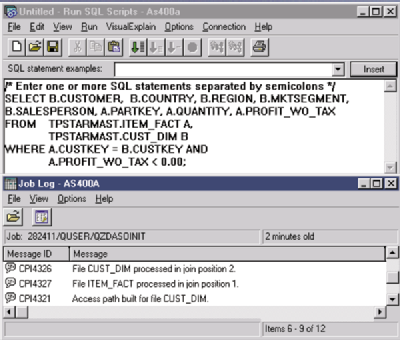
Figure 1: Visual Explain includes windows for an SQL statement and the job log.

Figure 2: Visual Explain shows all steps needed to satisfy an SQL query.

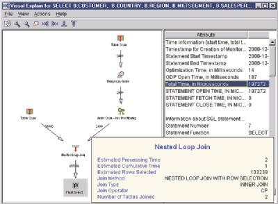
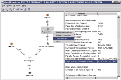
Figure 3: Visual Explain allows you to create an index on the fly.

Figure 4: Creating an index for the join condition reduces run time.

Figure 5: Visual Explain suggests creating an index based on the WHERE clause.

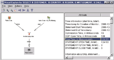
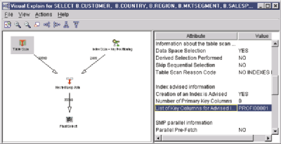
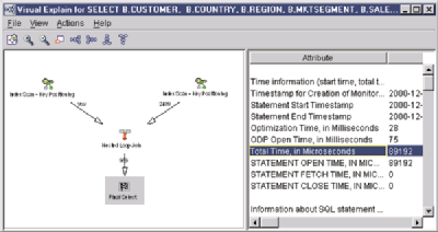
Figure 6: Creating a second index further improves performance.

Also Read

Practical Middleware: Starting the Journey

IBM i 7.2: The Carrot Versus the Stick

A Renaissance for Domino