You may recall that in earlier articles of this series, we saw that artificial intelligence (AI), machine learning (ML), and deep learning (DL) are technologies that are primarily used to analyze immense volumes of data to find common patterns that can be turned into actionable predictions and insights. Read Part 1, Understanding Data and Part 2: Artificial Intelligence, Machine Learning, and Deep Learning.

However, as data generation and collection grows, drawing inferences from the data available becomes more and more challenging. It’s not unheard of to have data sets with hundreds or even thousands of columns (dimensions) and millions of rows. And, the more dimensions you have, the more combinations of data you need to examine to find patterns amongst all the possible combinations of data available. That’s why reducing the total number of dimensions used is vital.

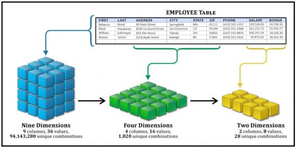
Figure 1: Dimensionality reduction

As the name implies, dimensionality reduction refers to the process of reducing the number of dimensions (features) found in a data set – ideally without losing too much information while keeping (or better yet, improving) model performance. As the example in Figure 1 illustrates, when unnecessary dimensions (or features) are eliminated, the number of possible combinations and permutations that must be analyzed is reduced – sometimes substantially.

As the number of dimensions used increases, ML and DL models become more complex. And the more complex a model is, the more the chances that overfitting will take place. Overfitting and underfitting are covered in more detail a little later, but in essence, overfitting occurs when a model is trained on so many features that it gets increasingly dependent on the data it was trained on and, in turn, delivers poor performance when presented with new, unknown data.

While avoiding overfitting is a major motivation for dimensionality reduction, there are several other advantages this effort provides:

• Less storage space is needed
• Redundant features and noise can be reduced or eliminated
• Less computing resources are needed for model training
• Models can be trained faster
• Model accuracy can be improved (because less misleading data is available during the training process)
• Simpler model algorithms (that are unfit for large numbers of dimensions) can be used

Dimensionality reduction can be done in two different ways: by keeping only the most relevant variables found in the original data set (this technique is called feature selection). Or by considering the data set as a whole and mapping useful information/content into a lower dimensional feature space (this technique is called feature extraction). Feature selection can be done either manually or programmatically; often features that are not needed can be identified just by visualizing the relationship between the features and a model’s target variable. For example, if you are trying to build a model that predicts the likelihood that someone will become diabetic and you have a column in your data set that contains eye color information, that information is probably not needed.

Feature extraction, on the other hand, is typically done programmatically. Programmatic methods for feature selection that are available with the popular ML library scikit-learn include variance threshold, which drops all features where the variance along a column does not exceed a specified threshold value, and univariate selection, which examines each feature individually to determine the strength of the relationship of the feature with the response variable.

Some feature extraction methods that rely on what is known as linear transformations. (A linear transformation is a mapping of a function between two modules that preserves the operations of addition and scalar multiplication.) Feature extraction techniques that rely on this methodology include:

• Principal Component Analysis (PCA): A technique which reduces the dimension of the feature space by finding new vectors that maximize the linear variation of the data. (The newly extracted variables are called Principal Components.) PCA rotates and projects data along the direction of increasing variance; features with the maximum variance become the Principal Components. PCA can reduce the dimension of the data dramatically without losing too much information when the linear correlations of the data are strong. (It can also be used to measure the actual extent of information loss and adjust accordingly.) PCA is one of the most popular dimensionality reduction methods available.
• Factor Analysis: A technique that is used to reduce a large number of variables by expressing the values of observations as functions of a number of possible causes to determine which are the most important. The observations are assumed to be caused by a linear transformation of lower dimensional latent factors and added Gaussian noise.
• Linear Discriminant Analysis (LDA): A technique that projects data in a way that class separability is maximized. Examples from the same class are put closely together by the projection; examples from different classes are placed far apart.

Non-linear transformation methods or manifold learning methods are used when the data doesn’t lie on a linear subspace. The most common non-linear feature extraction methods include:

• t-distributed Stochastic Neighbor Embedding (t-SNE): Computes the probability that pairs of data points in the high-dimensional space are related and then chooses a low-dimensional embedding that produces a similar distribution.
• Multi-Dimensional Scaling (MDS): A technique used for analyzing the similarity or dissimilarity of data as distances in a geometric space. MDS projects data to a lower dimension such that data points that are close to each other (in terms of Euclidean distance) in the higher dimension are close in the lower dimension as well.
• Isometric Feature Mapping (Isomap): Projects data to a lower dimension while preserving the geodesic distance (rather than Euclidean distance as in MDS). Geodesic distance is the shortest distance between two points on a curve.
• Locally Linear Embedding (LLE): Recovers global non-linear structure from linear fits. Each local patch of the manifold can be written as a linear, weighted sum of its neighbors, given enough data.
• Hessian Eigenmapping (HLLE): Projects data to a lower dimension while preserving the local neighborhood like LLE but uses the Hessian operator to better achieve this result (hence the name). In mathematics, the Hessian matrix is a square matrix of second-order partial derivatives of a scalar-valued function or scalar field.
• Spectral Embedding (Laplacian Eigenmaps): Uses spectral techniques to perform dimensionality reduction by mapping nearby inputs to nearby outputs. It preserves locality rather than local linearity.

It’s not important that you understand exactly how the dimensionality reduction methodologies presented here work – that falls under the domain of a data scientist. However, it is good to be aware of some of the names of the more common methods used, which is why they are presented here.

Data preparation – data splitting

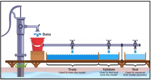
Figure 2: Data splitting

Ultimately, the goal of ML and DL is to create computational models that can make data-driven decisions or predictions that prove to be accurate most of the time. These models are created through a process called “training”, which involves teaching algorithms to look for patterns in “training data” that can be used to map input attributes to output targets. (As we saw in the previous article in this series, the term model refers to the artifact that is created by the training process.) Trained models are then evaluated by comparing predictions made on an “evaluation” data set with true values (known as ground truth data) using a variety of metrics. Then, the “best” model is used to make predictions on future instances for which the target answer is unknown.

Of course, a model should not be evaluated with the same data that’s used to train it – such an approach can reward models that “remember” the training data, as opposed to making correct generalizations from it. Consequently, most data scientists divide their data (that is, historical data that contains both input attributes and known output targets) into three different data sets:

• A training data set: Data that contains the set of input examples the model is to be trained on (or “fit” to). The model sees and learns from this data.
• A validation data set: Data that is used to provide an unbiased evaluation of a model repeatedly, as it is tuned. Data scientists use this data to fine-tune the model’s hyperparameters, over multiple iterations. (More information on hyperparameters will be provided shortly.) Consequently, the model sees this data occasionally, but never learns from it. It’s important to keep in mind that with each iteration, a model’s evaluation will become more biased as information obtained from the validation process is incorporated back into the model to make it better fit both the training data set and the validation data set.
• A test data set: Data that will be used to provide an unbiased evaluation of the final model that has been fit to the training data set. This data set provides the “gold standard” that is used to evaluate the final model and is only used after all model training and tuning is complete. The test data set is generally well curated and often contains carefully sampled data that spans the various classes the model would most likely encounter when used in the real world.

So, how is data usually split to create these three data sets? Typically, the bigger the training data set, the better, but the answer really depends on two things: the total number of samples (that is, input attributes and known output targets) in the full data set available and the task the model being trained is intended to perform. Complex models that need a substantial amount of data for training will require a very large training data set. On the other hand, models with very few hyperparameters that will be relatively easy to validate and tune, might be able to take advantage of smaller data sets for validation and test. If you have a model that doesn’t contain hyperparameters or that can’t be easily tuned, you might not want a validation data set at all.

Like many things in ML and DL, the training-validation-test split ratio is specific to individual use cases. And, as you gain experience building and training models, it will become easier to make the right decisions. That said, a common strategy is to take all available data and split it using a ratio of 70-80% for training and 20-30% for validation and test, with the latter amount being split evenly between the two.

A word about Cross Validation

Sometimes, people will split their data set into just two data sets – training and test. Then, they set aside the test data set, and randomly choose X% of their training data set to be the actual training set used and the remaining (100-X)% is used as the validation data set, where X is a fixed number (say 80%). The model is then iteratively trained and validated on these different sets. This approach is commonly known as cross validation because basically, the initial training data set created is used to generate multiple splits of the training and validation data sets used. Cross validation avoids over fitting and is becoming more and more popular, with K-fold Cross Validation being the most popular method used.

Underfitting and overfitting

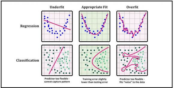
Figure 3: Underfit, appropriate fit, and overfit

Arguably, ML (and DL) models have one sole purpose and that is to generalize well. That is, to provide sensible outputs or accurate predictions when presented with input data they’ve never seen before. The term generalize refers to the ability to form general concepts from just a few facts, by abstracting common properties. For example, if you know what a cat looks like, you can easily identify a cat in a photograph, regardless of its color, size, location in the picture, or orientation of the photograph itself. That’s because humans generalize with incredible ease. ML models, on the other hand, struggle to do these things. A model trained to identify cats in images positioned right side up might not recognize a cat at all in an image of one that has been turned upside down.

From an ML perspective, there are essentially two types of data points: one that contains information of interest, known as the signal or pattern, and another that consists of random errors, or noise. Take for example, the price of a home. Aside from location, home prices are largely dependent upon the size of the lot a home sits on, the square footage of the home itself, the number of bedrooms the home has, and so forth. All of these factors contribute to the signal. Thus, a larger lot size or more square footage typically leads to a higher price. However, houses in the same area that have the same lot size, same square footage, and same number of bedrooms do not always have the same sales price. This variation in pricing is the noise.

To generalize well, an ML model needs to be able to separate the signal from the noise. However, it can be challenging to construct an ML model that is complex enough to capture the signal or pattern you’re looking for in data, but not so complex that it starts to learn from the noise. That’s why many ML models fall prey to what is known as overfitting and underfitting.

Overfitting refers to an ML model that has learned too much from its training data. Instead of finding the signal or dominate trend, the model ends up treating noise or random fluctuations as if they were intrinsic properties of the data. Consequently, the concepts the model learns are not applicable to new, unseen data so its generalization is unreliable. Like a student who has memorized all the problems in a textbook, only to find themselves lost when presented with different problems on an exam, an overfit model will perform unusually well when presented with the training data itself, but very poorly when given data it has not seen before.

Overfitting occurs when a model is either too complex or too flexible; for example, if it has too many input features or it has not been properly regularized. (Regularization refers to a broad range of techniques that can be used to artificially force a model to be simpler.) Some methodologies that are used to avoid overfitting include:

• Collecting more data
• Choosing a simpler model
• Cross-validation (5-fold cross validation is a standard way of finding out-of-sample prediction errors)
• Early stopping, which is a technique for controlling overfitting when a model is trained using an iterative training method (such as gradient descent)
• Pruning, which is used extensively with decision trees and involves removing nodes that add little predictive power for the problem at hand.

Underfitting, the counterpart of overfitting, refers to an ML model that has not learned enough from its training data to accurately capture the underlying relationship between input data and target variables. Such models can neither predict the targets in the training data sets very accurately nor generalize to new data. Underfitting occurs when an excessively simple model is used, when there is not enough training data available to build a more accurate model, or when a linear model is trained with non-linear data. It can be avoided by using more training data and/or reducing feature selection.

Both overfitting and underfitting result in models that deliver low generalization and unreliable predictions. Thus, underfitting and overfitting can often be detected by comparing prediction errors on the training data used with errors found with evaluation data.

Model parameters and hyperparameters

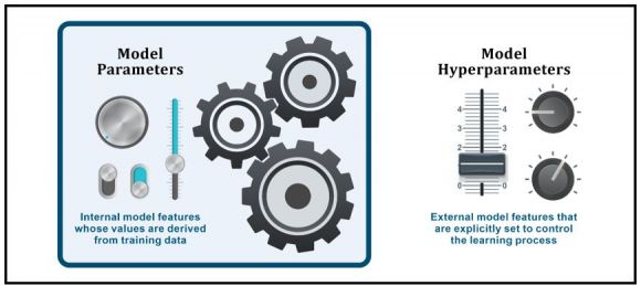
Figure 4: Model parameters and hyperparameters

An unfortunate quirk of computer science terminology is that specific terms are sometimes used interchangeably. For example, in programming, the terms parameters and arguments are frequently used synonymously, even though, in the strictest sense, they have distinct meanings. Arguments are the actual values passed in a function call while parameters are the placeholders in a function definition that receive the values passed. The same is true in machine learning when it comes to the terms parameter and hyperparameter.

One of the toughest challenges data scientists face when implementing AI solutions is model optimization and tuning. So much so, that entire branches of ML and DL theory have been dedicated to this subject. Typically, we think of model optimization as a process of regularly modifying a model to minimize output error or improve model accuracy. However, ML and DL model optimization often entails the fine tuning of elements that live both inside and outside the model.

A model parameter is a configuration variable that is internal to a model – parameters are a part of a model that is learned from the training data. Therefore, parameters values are typically NOT manually set by a data scientist. Instead, they are estimated using an optimization algorithm, which is a type of efficient search through possible parameter values. Parameters are often saved as part of a model and may be required by the model when making predictions. Examples of model parameters include:

• The weights in an artificial neural network (we will look at neural networks in another article in this series)
• The support vectors in a Support Vector Machine (SVM)
• The weight coefficients in a linear regression model

A model hyperparameter, on the other hand, is a configuration element that is external to a model that can heavily influence its behavior. Unlike model parameter values, model hyperparameter values cannot be estimated from training data. Instead, they are explicitly specified by a data scientist (however, they can be set using heuristics) and are often tuned for a given predictive modeling problem. They may also be used in processes to help estimate model parameter values.

Basically, hyperparameters help with the learning process. They don’t appear in the final model prediction, but they have a huge influence on how parameters will look after the learning step. Some examples of model hyperparameters include:

• The learning rate for training a neural network
• The number of distinct clusters to use with K-Means clustering
• The C and gamma parameters for a Radial Basis Function (RBF) kernel Support Vector Machine (SVM)

Stay Tuned

In the next part of this article series, we’ll explore the different types of machine learning that’s available and we’ll explore some of the different parameters and hyperparameters just described.

Roger E. Sanders is a Principal Sales Enablement & Skills Content Specialist at IBM. He has worked with Db2 (formerly DB2 for Linux, UNIX, and Windows) since it was first introduced on the IBM PC (1991) and is the author of 26 books on relational database technology (25 on Db2; one on ODBC). For 10 years he authored the “Distributed DBA” column in IBM Data Magazine, and he has written articles for publications like Certification Magazine, Database Trends and Applications, and IDUG Solutions Journal (the official magazine of the International Db2 User's Group), as well as tutorials and articles for IBM's developerWorks website. In 2019, he edited the manuscript and prepared illustrations for the book “Artificial Intelligence, Evolution and Revolution” by Steven Astorino, Mark Simmonds, and Dr. Jean-Francois Puget.

From 2008 to 2015, Roger was recognized as an IBM Champion for his contributions to the IBM Data Management community; in 2012 he was recognized as an IBM developerWorks Master Author, Level 2 (for his contributions to the IBM developerWorks community); and, in 2021 he was recognized as an IBM Redbooks Platinum Author. He lives in Fuquay Varina, North Carolina.

---

MC Press books written by Roger E. Sanders available now on the MC Press Bookstore.

		QuickStart Guide to Db2 Development with Python Discover how Python, SQL, and Db2 can successfully be used with each other. List Price $9.95 Now On Sale
		DB2 10.5 Fundamentals for LUW (Exam 615) Don't even think about attempting to take the DB2 Fundamentals exam without this indispensable study guide. List Price $79.95 Now On Sale
		DB2 10.1 Fundamentals (Exam 610) Let one of the world's leading DB2 authors and a participant in the exam development help you succeed. List Price $79.95 Now On Sale
		Artificial Intelligence: Evolution and Revolution Operational AI has become available to the masses, setting the wheels in motion for a worldwide AI revolution that has never been seen before. List Price $16.95 Now On Sale
		DB2 10.5 DBA for LUW Upgrade from DB2 10.1: Certification Study Notes Here's everything you need to know to take and pass Exam 311, complete with a practice exam and study key. List Price $21.95 Now On Sale
		From Idea to Print Here's everything you need to know to turn your technical knowledge and expertise into a published article or book. List Price $49.95 Now On Sale
		DB2 9 Fundamentals (Exam 730) Use this review before taking the test to prove you've mastered the basics of DB2 9. List Price $59.95 Now On Sale
		DB2 9 for Linux, UNIX, and Windows Database Administration (Exam 731) Use this indispensable study guide to prepare to take, and pass, Exam 731. List Price $64.95 Now On Sale
		DB2 9.7 for Linux, UNIX, and Windows Database Administration (Exam 541) Get ready to take the DB2 9.7 certification exam with this handy study guide. List Price $21.95 Now On Sale
		DB2 9 for Linux, UNIX, and Windows Advanced Database Administration (Exam 734) Review all exam topics and take the included practice test to be sure you're ready on testing day. List Price $64.95 Now On Sale
		DB2 9 for Linux, UNIX, and Windows Database Administration Upgrade (Exam 736) Prep for success with the master of DB2 certification study guides! List Price $34.95 Now On Sale
		Data Fabric: An Intelligent Data Architecture for AI This book explains the concepts and values that a data fabric approach can deliver to both technical and business communities. List Price $19.95 Now On Sale

Also Read

How AI Will Stoke Rather Than Dampen Job Markets

Putting the Brakes on the AI “Runaway Train” Myth

Artificial Intelligence, Part 6: Measuring Quality and Understanding Challenges