


Having AQP is like having "quality control" inside your query plans.
According to Wikipedia, "adaptive behavior" is a type of behavior that is used to adjust to another type of behavior or situation. This is often characterized by a kind of behavior that allows an individual to change an unconstructive or disruptive behavior to something more constructive.
DB2 for i, the powerful database management system integrated into IBM i, has the distinction of possessing this adaptive characteristic for SQL queries. Adaptive query processing, or AQP, has really come into its own in the latest version of IBM i. For years, DB2 for i has been known for ease of use, low total cost of ownership, and unique capabilities aimed at solving business problems. Version 7 Release 1 of IBM i extends these positive qualities by providing an insurance policy for particularly thorny requests—namely, join queries that have complex predicates, seemingly simple predicates referencing data sets with skewed or non-uniform row distributions, or situations where good statistics are just not available at run time.
Query Optimization Revisited
Simply put, optimization is the act of evaluating a query request and determining the best plan based on the SQL syntax, the data, and the environment. In reality, there are many factors or variables that go into the process. See Figure 1.
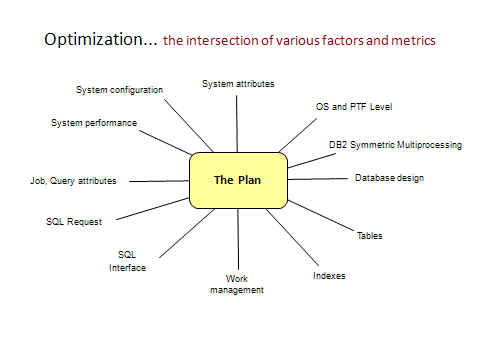
Figure 1: Multiple factors must be considered in the process of optimization.
During the process, the query optimizer is looking for the strategy and methods that will result in the most efficient use of CPU time and I/O processing—in other words, the fastest plan. To do this, fixed costs are considered, things like the number and relative speed of the processors, the amount of memory available, and the time to read from disk and write to disk. The optimizer implicitly knows about the properties of database objects: table size, number of rows, index size, number of keys, etc. The optimizer can also determine some of the data attributes: cardinality of values in a column, distribution of rows by value, relationships between rows in one table and another table given a specific column comparison. The presence of database constraints can also be helpful. It is precisely the data attributes and relationships that can be troublesome and cause an otherwise good query to go bad. Using an index or column statistic to determine the number of distinct colors represented in a table is easy and straightforward, as in confidently estimating the number of rows that have the value of 'BLUE'. But what about estimating the number of rows in a table where order arrival date is greater than order date plus 31 days or order arrival date minus order ship date is greater than 10 days? It is much more difficult to determine answers based on these types of "data interdependencies" without actually running a query to understand the data.
To further appreciate the effort involved in query optimization, consider the tables containing customers, orders, items, and shipping metrics. See Figure 2.
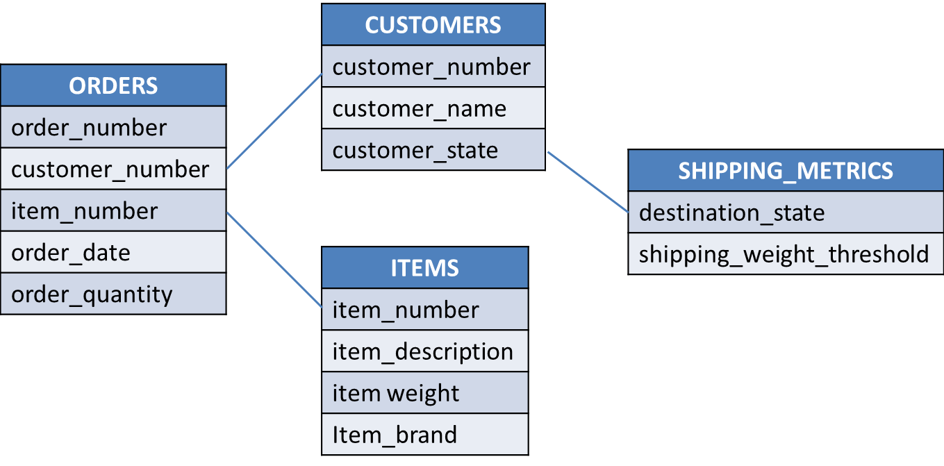
Figure 2: Let's use these tables as an example. (Click images to enlarge.)
On average, each customer has 100 orders. And on average, each item has 1,000 orders. When looking at the data in the orders table, each customer will generally be represented 100 times, and each item will generally be represented 1,000 times. In other words, 100 orders will have the same identical customer number value, and 1,000 orders will have the same identical item number value. Also assume that the master tables containing customers and items respectively have no duplicate identification numbers; each customer column value and item column value is unique within the associated master table.
A user's query might state something like this: for a given set of customers and a given set of items, find the associated orders where the item weight is greater than a specified threshold (a situation where shipping costs might be higher than normal).
SELECT c.customer_state,
c.customer_number,
c.customer_name,
o.order_number,
o.order_date,
o.order_quantity,
i.item_number,
i.item_brand,
i.item_description,
i.item_weight
FROM orders o
INNER JOIN customers c
ON o.customer_number = c.customer_number
INNER JOIN items i
ON o.item_number = i.item_number
WHERE c.customer_state IN ('IA', 'IL', 'MN')
AND i.item_brand = 'BIG BAD MACHINES'
AND (i.item_weight / 2204.6) >=
(SELECT s.shipping_weight_threshold
FROM shipping_metrics s
WHERE s.destination_state = c.customer_state)
ORDER BY c.customer_state,
c.customer_name,
c.customer_number
OPTIMIZE FOR 20 ROWS;
To find the set of orders, the database request would consist of joining a customer master row with the 100 (on average) related rows from the orders table, or joining the item master row with the 1,000 (on average) related rows from the orders table, and then joining the particular order row to the table of shipping metrics by state. But what if one particular customer or item had 100,000 orders? Or no items have a weight greater than the shipping threshold? The optimizer's assumptions and understanding about the relationships and join processing could be off by several orders of magnitude, possibly resulting in a very poor query plan. In other words, the data within the orders table is skewed where a particular value for customer number or item number represents a very large set of data or no data at all. During query optimization, this situation can go undetected unless the optimizer has some special statistics about the column values or the optimizer actually runs the query and uses the results to better understand the data.
Speaking of understanding the data, the DB2 for i query optimizer can make use of indexes as well as column statistics, provided they exist. If an index and/or a column statistic covers the respective join columns of each table and the local selection predicates, the optimizer will have a high probability of identifying and building the best plan. But what if the indexes do not exist? Or what if the local selection predicate is too complex to calculate and store prior to running the query? The query optimizer will use default values and probability calculations for the selectivity and join predicates. If the default values happen to match the attributes of the data, then as luck would have it, the query plan will be adequate. If not, the optimizer's plan will likely be suboptimal and a poor performer. The best way to minimize this situation is to identify and implement an adequate indexing strategy.
Query Implementation Choices
Given the previous SQL request, the most basic and logical options for join position are shown in Figure 3.
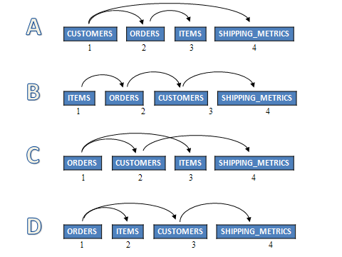
Figure 3: These are the most logical join options for our example.
In example A, the customer rows are read first (table 1). It uses the WHERE clause predicate so that only customers from the states 'IA', 'IL' and 'MN' will be selected. The customer number will be used to find the associated orders in table 2. If an order is found, the item number from the order will be used to find the item attributes (brand and weight) in table 3. To complete the test, the state value from the customer row is used to locate the shipping metrics whereby the item weight is compared to the shipping weight threshold in table 4. Not until all of the tests are performed successfully and positively across the tables will a row be returned from the join processing.
In example C, the orders are read first (table 1). Because the query specifies no local selection on orders, every row must be read and joined in turn to customers (table 2) to determine if the order is selected. If the matching customer row contains one of the three state values specified, then the items table is read using the item number from the orders table. If the matching item row contains the brand specified, then the item's total weight is compared against the customer's state shipping threshold in table 4. This scenario might make good sense if the query is expected to select most or all of the orders.
The best and most efficient join order will depend on which first pair of tables reduces the query's result set the fastest. In other words, if there are few rows in the customers table where column customer_state equals 'IA' or 'IL' or 'MN', and customer is the first table in the join followed by the orders table, then the query will be completed very quickly with little effort. On the other hand, if the orders table is first, followed by the customers table, then all the order rows will be read. Each order will have to be used to look up the corresponding customer row, where the test on state will be performed. If the customer's state does not meet the local selection criteria, the query will require much more I/O, processing, and time to produce little or no results. But what if the great majority of orders are from customers located in Iowa, Illinois, or Minnesota? Having the orders table first, followed by the customers table or even items table might be very productive. The net of this is that the join order—i.e., the relative order in which the tables are accessed—matters greatly. And getting the join order correct depends on understanding the relative selectivity of WHERE clause predicates and the relationships between each table's join column values.
Adaptive Query Processing
It would be wonderful if the query optimizer had all of the relevant information and processing options before handling the query, resulting in the best plan and performance on the first iteration. In reality, this is either improbable or impossible for many complex SQL requests. Thus, come to expect a really bad query from time to time based solely on this first iteration. When this occurs, plan on canceling any long-running unproductive requests, seek to analyze the query behavior, and try to provide more information to the optimizer. Unfortunately, this means paying the price for the bad run and relying on post-run exploration to hopefully improve future runs.
What if the database system did some or all of this work? What if, during the initial run of the complex query, the system recognized the query plan was unproductive and then intervened? That would be wonderful! Well, this is exactly what AQP, adaptive query processing, is all about: the ability of DB2 for i to watch, learn, and react by adapting to the data and environment. This allows unconstructive query behavior to be changed to be more constructive.
There are two main scenarios in which AQP can assist: during query execution and after query execution. This means that while the query is running, AQP can get involved to make it better, or after the query is completed, AQP can make use of the run-time metrics and query results to do a better job next time. See Figure 4.
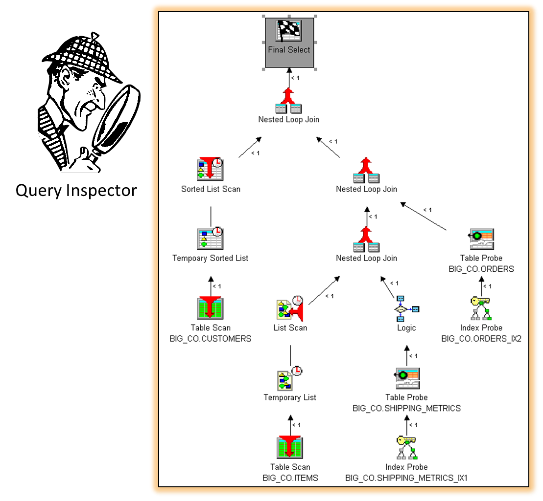
Figure 4: AQP watches and learns so that current and future queries perform better.
The components of AQP consist of:
- Current query inspector
- Query plan cache
- Query plan inspector
- Global statistics cache (GSC)
The current query inspector is responsible for watching the execution of a query in real time and deciding when and how to react. Real-time inspections and analysis are not initiated until the query has been executing for at least two seconds and the query has not returned any results to the requester. In other words, once the query has produced an answer and returned control to the application, AQP cannot get involved as this would change the answers. Currently, real-time AQP is focused only on SQL queries that reference more than one table—e.g., joins, subqueries, common table expressions, derived tables, etc. During the query's execution, AQP spawns a secondary thread to watch for unproductive joins, inaccurate or misleading row count estimates, and any new and useful indexes that have been created. After some analysis and learning, AQP can initiate a query optimization—while the current query continues to run. Think of this as a race; will the query produce results before the optimizer finds a better plan? If the new plan is deemed better than the current plan, and the current query has still not produced any results, then the current query is terminated and the new plan is started in its place, all within the same job. This process is totally transparent to the user's application. The new plan and the fact that AQP produced it will be saved in the plan cache. See Figures 5 and 6.
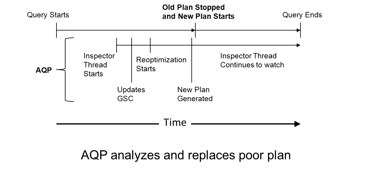
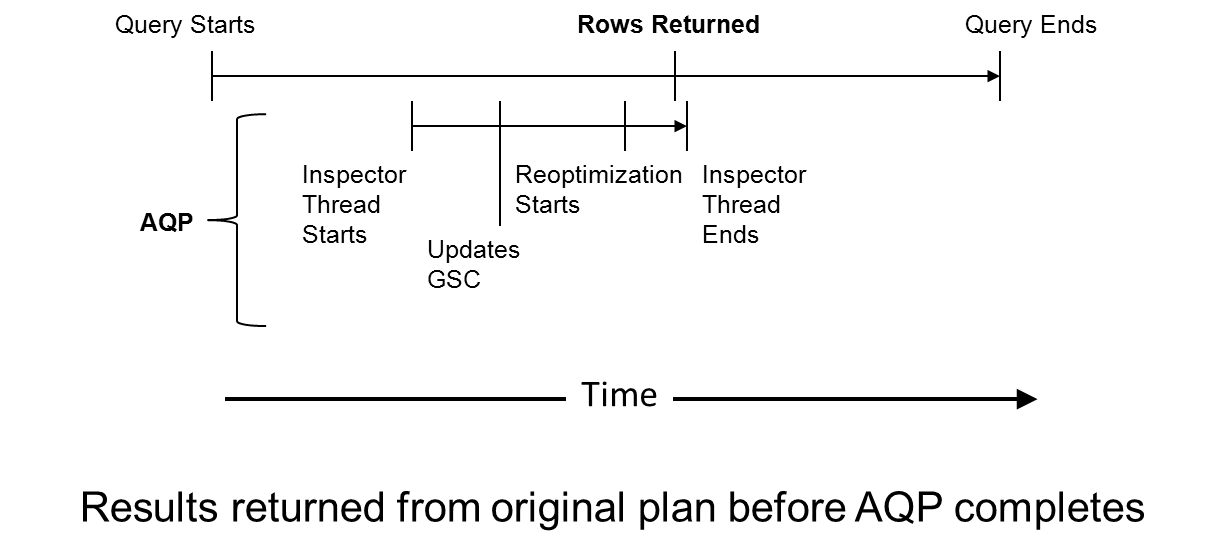
Figures 5 and 6: AQP watched and determined that there was a better way!
The query plan cache is a self-managed system-wide repository for all SQL query plans. After query optimization, the query plan is saved in the plan cache. During and after query execution, run-time metrics are accumulated and saved with the respective plans. Both the query plan and metrics can be used to minimize or eliminate time and effort on future runs.
The plan cache inspector analyzes existing plans in the plan cache over time. The analysis involves comparing row counts and run-time estimates to actuals, taking note of computed values from complex predicates, as well as understanding the performance attributes of particular join orders. Particularly thorny plans can be marked for deeper analysis. The positive result of inspecting plans is learning and optimizing future query plans based on the previous query execution and system behavior. This is yet another example of DB2 for i self-tuning.
The global statistics cache (GSC) is a self-managed system-wide repository for complex statistics. As AQP is watching real-time queries or inspecting plans in the cache, information is gleaned and documented in the GSC. This is part of the learning componentry used to enhance query optimization over time. See Figure 7.
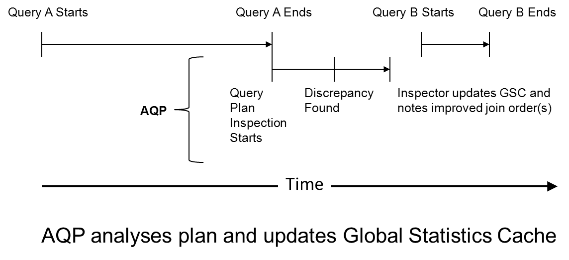
Figure 7: AQP performs its analysis and updates the GSC.
Examples of AQP in Action
Using the four tables and SQL previously described, here are a few scenarios in which AQP can add value by taking a long-running, unproductive query and revitalizing it in real time.
In this first example, the initial plan has a poor inner join scheme with the customers table first, followed by the orders table. Three tables are continually being read without any matching rows found for further processing. The query is "stuck" in the first phase of the join and is subsequently starving the rest of the query plan. This results in a long run time with no results being produced for the requester. See Figure 8.
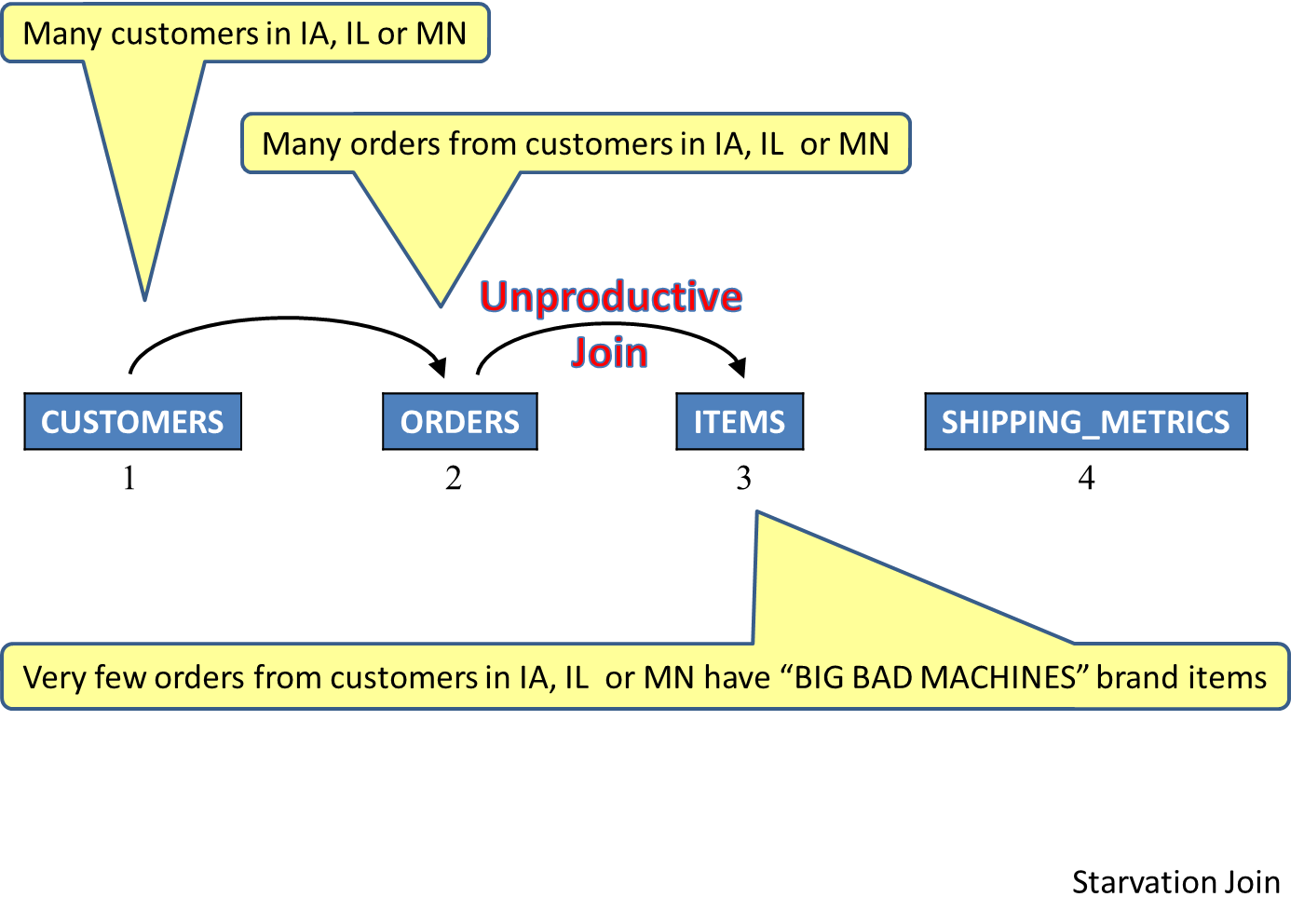
Figure 8: This inner join scheme is unproductive.
After two seconds, AQP begins to watch the query's behavior and decides to build a new plan with a different join order. The new plan places the items table first, orders table second, and customers table third as it appears that the number of orders with the selected item brand is low. Thus fewer rows will be referenced in the orders table, and these rows are likely to produce results. See Figure 9.
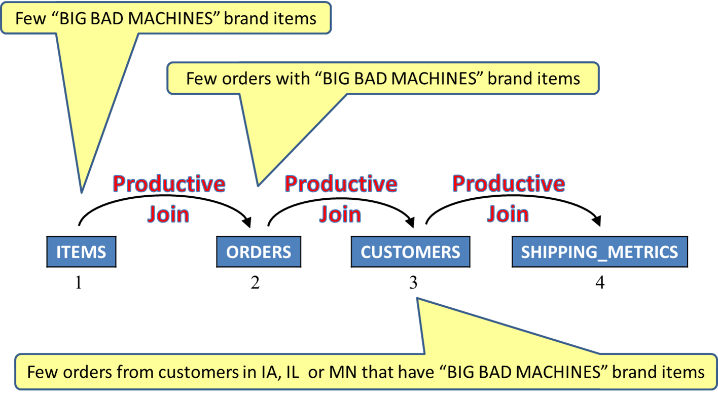
Figure 9: This join scheme will now produce results much more quickly.
In this second example, the initial plan has the ORDER BY criteria pushed down, resulting in a join order with customers table first. This allows customers to be read via an index with key columns: customer_state, customer_name, customer_number. This delivers the customers table rows in the proper order and preserves that order as the join portion of the query is processed. It also helps to support the optimization goal of 20 rows. In other words, the application wants the first 20 query results as fast as possible. Unfortunately, this join order might also result in an overall worse-performing query. In other words, efficient join processing is sacrificed in favor of ordering efficiency. See Figure 10.
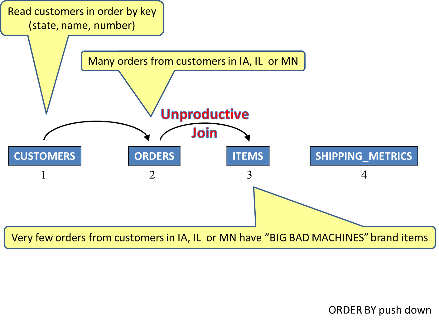
Figure 10: The ordering scheme causes a poor join order.
After two seconds, AQP begins to watch the query's behavior. A new optimization without the ORDER BY pushed down to the primary table results in a different join order. The new plan places the items table first, orders table second, and customers table third as it appears that the number of orders with the requested brand is low. The selection and join processing will improve, and the ordering will be accomplished via a sort instead of an index. Given the relatively small number of results expected, the overall query performance is much better even for an optimization goal of 20 rows. See Figure 11.
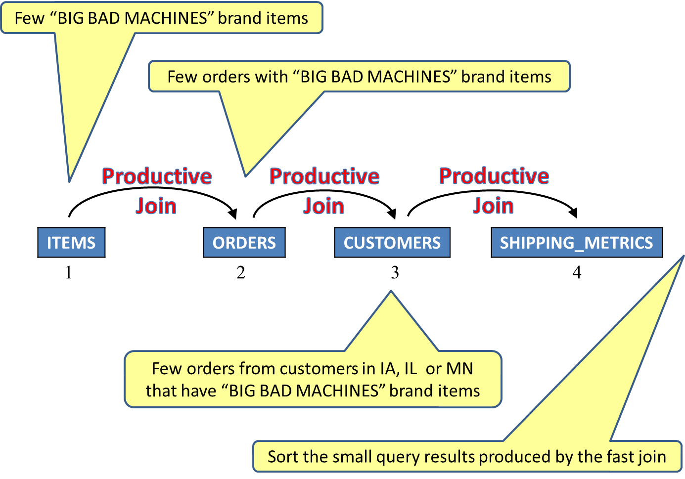
Figure 11: AQP removed the ordering based on the first table and freed up the join order.
In the third example, the initial plan has an acceptable join order, but is not meeting expectations. This is due to the orders matching the brand criteria but not matching the state criteria. If it were possible to recognize and apply both the brand and state criteria to the orders table at once, then the join order will not matter as much. This new strategy will be based on DB2 for i discovering and applying local selection to the orders, which has no local selection specified in the SQL statement. By using both the customers table and the items table via a technique known as "look-ahead predicate generation," or LPG, the orders table can be accessed using a relative row number list produced by two indexes with key columns of item_number and customer_number, respectively. This means only the orders that have a match in the items table and customers table will be selected! In effect, the orders table can be placed first in the join order, and selection and joining will be most efficient. See Figure 12.
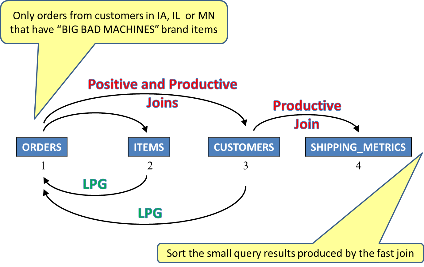
Figure 12: AQP has developed a fast, efficient, productive plan!
What to Do and What to Expect
In laboratory tests, the positive effects of AQP show up when running complex queries that have moderate to little tuning via indexes. It is also beneficial where the query has derivatives and/or calculations in the predicates, as well as when the data is highly skewed or has hidden correlations. In these cases, the intervention by AQP turns a very tardy result into a set of prompt answers. For simple or well-tuned queries, the optimizer does a great job of identifying the best plan, thus AQP does not usually get invoked, or it plays a limited role. Adaptive query processing can be thought of as an insurance policy against misunderstood data and unexpected behavior.
How do you take advantage of this exciting and valuable feature? Move up to IBM i 7.1! AQP is automatic and available for all SQL queries. There is no user intervention or management required. If AQP does get invoked for a query, this fact is documented and available via analysis tools such as Visual Explain and the SQL Performance Monitor.
If you are still shying away from SQL queries and assume a high-level language program with native record level I/O is better and faster, picture this: a user is running your program and waiting for results. Waiting and waiting and waiting. You, the programmer, notice the unproductive program behavior, analyze the situation, rewrite the logic, compile the code, and slip in the new program—all without the user's knowledge or intervention. This is Adaptive Query Processing, and it is available now, with SQL and DB2 for i.
as/400, os/400, iseries, system i, i5/os, ibm i, power systems, 6.1, 7.1, V7, V6R1


 More than ever, there is a demand for IT to deliver innovation. Your IBM i has been an essential part of your business operations for years. However, your organization may struggle to maintain the current system and implement new projects. The thousands of customers we've worked with and surveyed state that expectations regarding the digital footprint and vision of the company are not aligned with the current IT environment.
 TRY the one package that solves all your document design and printing challenges on all your platforms. Produce bar code labels, electronic forms, ad hoc reports, and RFID tags – without programming! MarkMagic is the only document design and print solution that combines report writing, WYSIWYG label and forms design, and conditional printing in one integrated product. Make sure your data survives when catastrophe hits. Request your trial now! Request Now.
 Forms of ransomware has been around for over 30 years, and with more and more organizations suffering attacks each year, it continues to endure. What has made ransomware such a durable threat and what is the best way to combat it? In order to prevent ransomware, organizations must first understand how it works.
 Disaster protection is vital to every business. Yet, it often consists of patched together procedures that are prone to error. From automatic backups to data encryption to media management, Robot automates the routine (yet often complex) tasks of iSeries backup and recovery, saving you time and money and making the process safer and more reliable. Automate your backups with the Robot Backup and Recovery Solution. Key features include:
 Business users want new applications now. Market and regulatory pressures require faster application updates and delivery into production. Your IBM i developers may be approaching retirement, and you see no sure way to fill their positions with experienced developers. In addition, you may be caught between maintaining your existing applications and the uncertainty of moving to something new.
 IT managers hoping to find new IBM i talent are discovering that the pool of experienced RPG programmers and operators or administrators with intimate knowledge of the operating system and the applications that run on it is small. This begs the question: How will you manage the platform that supports such a big part of your business? This guide offers strategies and software suggestions to help you plan IT staffing and resources and smooth the transition after your AS/400 talent retires. Read on to learn:
LATEST COMMENTS
MC Press Online