In the first article in this series, you learned about modifications that you can make to Work Management in order to get jobs directed to different main storage pools. The article also explained how you can advise the automated tuning function of OS/400 to allocate storage to the different storage pools.

But are there additional changes you can make to improve the way work is done in the main storage pools? What is happening to the jobs that are running? How does the system decide which jobs should be run? If separating your jobs into different pools still hasn't produced the performance that you'd like, it's time to look at the answers to these questions and to see what adjustments, if any, you can make to get your jobs to run better. As before, this article will contain excerpts from iSeries and AS/400 Work Management. In this article, I will examine the following topics:

• Functions of the automatic tuning of OS/400
• Improving the paging characteristics of the pools the jobs are using
• Removing troublesome jobs from a storage pool
• OS/400 scheduling/dispatching
• Adjustments to a job's run priority

These techniques will provide you with additional Work Management adjustments that you can use to improve your system performance.

First, you need to look at what is happening in the pools where the jobs are running. To see what's going on, look at the WRKSYSSTS display. This display presents a lot of information regarding the current condition of your system (Figure 1).

Figure 1: The Work with System Status (WRKSYSSTS) display shows run-time information about your system. (Click images to enlarge.)

The content of this display is described in detail in Chapter 4 of iSeries and AS/400 Work Management. Rather than repeat all of the information, I will focus only on the values that pertain to this article:

• Database faults and pages
• Non-database faults and pages
• Max Act

Database Faults and Pages

I'll begin with the definition of a fault. A fault, or page fault, occurs whenever a job running in main storage requests a page of information that is not in main storage. The job that requests the page stops and waits for the page to be retrieved from disk. When the page has been retrieved and is ready for use, the job may resume processing. Because the job must stop and wait for the page to be read into main storage, keeping the number of page faults low is very important. Disk operations that force a job to stop and wait for the completion of the operation are called synchronous I/O operations. Whenever the system performs a synchronous operation, it tries to keep the number of pages read to a small number--usually 1 or 2 pages per fault. By keeping the number of pages transferred small, less overhead is required for reading them to main storage. As a result, the length of time the job is forced to wait is kept to a minimum.

The database fault value shows the number of times per second that the system stopped one of the jobs running in the pool while it retrieved a page from a database object for the job. The database pages value shows the number of pages per second that are being read into the pool. In the example, you see very little activity except for pool 2 (*BASE). In *BASE, you see a low DB fault value (2.0) and a very high DB pages value (257.5). But isn't the system supposed to bring a small number of pages on a fault? If so, why is the number of pages per fault more than 125? Good observation!

There is a good explanation for this apparent inconsistency. By analyzing the usage of database objects, the system support for database functions tries to anticipate what records and keys will be needed in main storage. As a good system citizen, database starts to read database pages into main storage before they are needed. Most of the time, database's read operations are complete before the job needs the data. Since a job does not need to wait for the disk operation to complete, there is no fault recorded for the I/O operation. These types of disk operations are referred to as asynchronous I/O operations.

Another factor that contributes to the large difference between faults and pages is database blocking. Whenever a job is processing a database file in the same sequence in which it is stored on disk, the job will run better if the application has implemented record blocking. Record blocking results in the transfer of large blocks of information from disk to main storage. And the system will perform these large block transfers asynchronously. This gives you the best of both worlds--large blocks with a single read operation that takes place while jobs keep running. So, when you see a low database fault value and a high database pages value, you can rest assured that the system database functions are hard at work on behalf of the jobs running on your system.

Non-Database Faults and Pages

These values represent the same information as the database values, except that these values represent faults and pages for any non-database objects. As you learned in the previous article, jobs running in a pool use information that is shared by other jobs and information that is unique to each job. Most of the non-database information read into a pool is job-unique information. There is usually little asynchronous activity for non-database objects. As a result, the fault and pages will have values that are close to the same. Once again, it is advantageous to keep the fault value low to reduce the number of times that a job must stop and wait for a disk operation. Trying to determine a reasonable number for the fault value will be discussed later in this article.

Max Active

Finally, we come to the last value, Max Active (maximum active). Maximum active does not restrict the number of jobs that can be initiated. Rather, it specifies the maximum number of threads that can be in main storage at the same time. There may be many more threads running on the system than are allowed into main storage.

An example will best explain this value. Many of you are familiar with registration for college classes. Often, many students are interested in the most popular courses. By accepting their registration, the registrar (subsystem) has processed their request (initiated the job). Using registration date (priority), the system begins to fill the class (allows jobs into main storage). When the class is full (all activity levels used up), no other students (jobs) are allowed into the class (pool). They are placed on a waiting list (ineligible) queue. If a student drops out of the class (job completes its work or reaches timeslice), one of the students on the waiting list is allowed into the class.

The simple diagram in Figure 2 shows the principles described above:
  

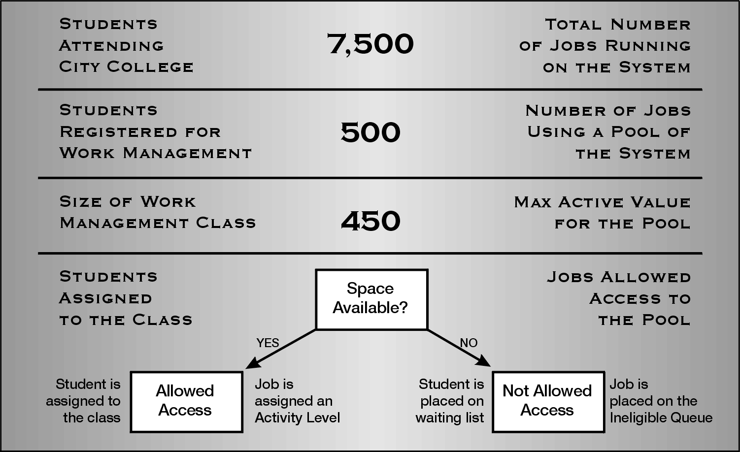
Figure 2: A pool's Max Active value is similar to the maximum number of seats in a class. 

If you look back at Figure 1, you'll notice the value of Max Active for the *MACHINE pool is +++++. What does that mean? Only low-level (Licensed Internal Code) system tasks will run in the *MACHINE pool. User jobs and most OS/400 system jobs run in the other pools. These low-level system tasks perform operations that are critical to the overall performance of the user jobs. Whenever a system task needs to run, it runs. System tasks are allowed immediate access to main storage no matter how many tasks are already in the *MACHINE pool. So, the +++++ is merely another way of saying that Max Active is not applicable to the *MACHINE pool.

While allowing an unlimited number of tasks access to the *MACHINE pool at the same time is acceptable, do not try this in any of the other pools. If too many jobs are running in a pool at the same time, there will be intense competition between the jobs for the space available in the pool. In particular, the jobs will be competing to get their unique information into main storage. As each job brings in more unique information, there is less room for shared information. As a result, there will be an increase in the number of faults for both job-unique and shared information. Finally, if the competition becomes too intense, a situation known as thrashing occurs. Simply stated, thrashing is a situation in which the system spends more time doing I/O operations than processing work. Thrashing results in horrendous performance!

OK. Nomax is not good. What is a good value for Max Active? What if I make Max Active for pool 3 really small, say 5? Would that be a good value? Well, maybe. Choosing the Max Active value depends on how frequently jobs want to access the pool. If a large number of jobs are always trying to get into main storage at the same time, setting Max Active too low will result in long waits on the ineligible queue.
So then, what is a good value for Max Active? Here's a simple method to determine a reasonable  activity level:

1. Pick a time of the day that represents your typical workload (if there is such a thing).
2. Reduce Max Active by 10%.
3. Continue to reduce Max Active by 10% until jobs are not allowed access to the pool--that is, they are placed on the ineligible queue.
4. When you see jobs on the ineligible queue, increase the activity level by 10%.
5. Monitor the ineligible queue periodically to validate your setting.

By using this simple technique, you will arrive at a reasonable setting for the Max Active value of your pools.

So, now you understand what this display means and why page faults are a detriment to performance. As you will recall from the first article, you use the WRKSHRPOOL command to set the initial pool sizes (Figure 3).

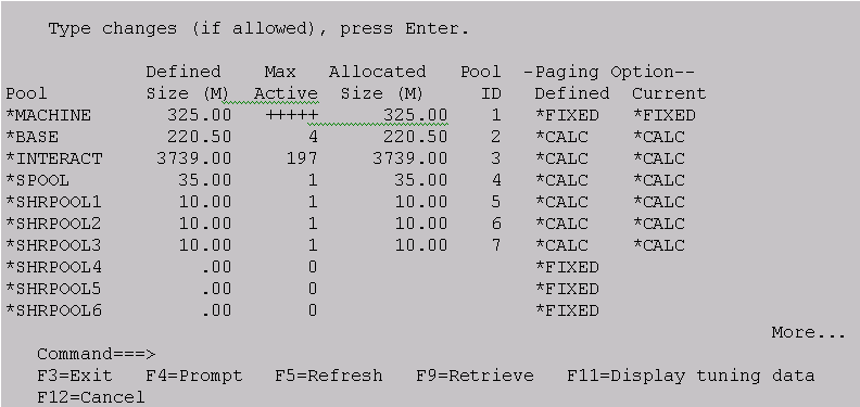
Figure 3: The first Work with Shared Pools display is used to provide initial pool sizes for the amount of main storage to be allocated to shared pools.

Dynamic Performance Adjustment

In order to make pool management easier, you can activate the dynamic performance adjustment functions of OS/400. Once activated, dynamic performance adjustment will attempt to balance storage between shared pools. It will also adjust activity levels in shared pools. In the default environment, all pools--*MACHINE, *BASE, *INTERACT, and *SPOOL--will be managed by the dynamic performance adjustment function.

Dynamic performance adjustment is controlled by the QPFRADJ system value. QPFRADJ can be set to the following: 

• 0--Do not initialize pool sizes, and do not dynamically adjust pool sizes and activity levels.
• 1--Initialize pool sizes when the system is IPLed (booted), but do not dynamically adjust pool sizes and activity levels.
• 2--Initialize pool sizes when the system is IPLed, and dynamically adjust pool sizes and activity levels.
• 3--Do not initialize pool sizes when the system is IPLed, but dynamically adjust pool sizes and activity levels

The default setting for QPFRADJ is 2.

So, when the system is IPLed, OS/400 will establish the initial size of all four pools. The initial sizes of the pools are calculated by an internal algorithm that analyzes the system resources, main storage size, processor speed, and installed features of OS/400. The algorithms are fixed and cannot be adjusted. In addition, when sizing the *MACHINE pool, OS/400 will consider the amount of reserved space that exists.

Once the pool sizes have been established, the IPL process continues. When IPL is complete, the susbsystems are active and are ready to initiate work into the pools. As you have learned, the initiated work will now begin to request information. Also, some of the requests will result in faults and force the user jobs to wait for the information. In  addition, there will be a system job, QPFRADJ, that is running. QPFRADJ, which is a system-initiated job (not via a subsystem), is the job that will perform the dynamic performance adjustments.

Estimating *MACHINE Pool Efficiency

I will focus my attention on the *MACHINE pool first. Unlike most of the other pools in the system, you shouldn't be concerned about the number of tasks that are running in this pool or the amount of CPU being used. The only thing you care about in *MACHINE is the page fault rate; nothing else matters. Every minute, QPFRADJ calculates the page fault rate in *MACHINE. If the page fault rate is less than 10, QPFRADJ is happy. If the page fault rate is greater than 10, QPFRADJ is disappointed (but not yet unhappy). If QPFRADJ finds the page fault rate of *MACHINE to be greater than 10 for three consecutive intervals, it becomes unhappy. Typically, most of your users will also be unhappy with the performance of their jobs.

In order to correct the high faulting rate in *MACHINE, QPFRADJ will increase the size of *MACHINE by changing the QMCHPOOL system value. QPFRADJ will increase the value of QMCHPOOL by 10%. Once QPFRADJ has started to increase the size of the *MACHINE pool, it will make an adjustment every minute until the page fault rate falls below 10.

There are three things to notice about QPFRADJ's management of high faulting in the *MACHINE pool:

1. The *MACHINE pool is always evaluated and adjusted first. As I mentioned earlier, the key components of the operation system are running in this pool. If these components are performing poorly, everything is performing poorly.

2. QPFRADJ waits for three consecutive intervals of poor faulting before any changes are made. Often, a small burst of transient activity may temporarily raise the faulting rate outside the 10 per second guideline. It is not advisable to adjust pool sizes when transient activities cause the faulting increase. The transient activities usually run quickly and faulting returns to a value of less than 10. By waiting for three intervals, QPFRADJ can be fairly certain the higher faulting rate is caused by normal activities.

3. Once QFRADJ has made an adjustment, it continues to adjust every minute. Since QPFRADJ has determined that the *MACHINE pool page faulting is caused by normal activities, high faulting in any subsequent interval is also considered to be caused by normal activities.

But, what happens if faulting in the *MACHINE pool never gets below 10? Hopefully, this condition will not happen in your environment. If it does, your system should be upgraded with additional main storage. In the meantime, QPFRADJ will try to distribute the main storage you have as evenly as possible. In the case of the *MACHINE pool, it means setting a maximum size. QPFRADJ will restrict the size of the *MACHINE pool to four times the reserved size of the pool. This size restriction prevents QPFRADJ from assigning all of your available main storage to the *MACHINE pool.

Up to now, I've addressed the situation of insufficient space in the *MACHINE pool. But, what would happen if there is too much main storage in the *MACHINE pool? QPFRADJ will not automatically reduce the size of QMCHPOOL; there must be a need for the storage in another pool. If all other pools in the system have too little storage, then storage will be taken from the *MACHINE pool and distributed to the other pools. Once again, QPFRADJ will not make any changes until the faulting condition has lasted for three intervals. Also, QPFRADJ will not reduce the size of *MACHINE below the minimum size of the *MACHINE pool--1.5 times the reserved size of *MACHINE.

Other Shared Pools

It would be nice if all you had to do was reduce *MACHINE pool paging in order to get your jobs to run well. But as you might have guessed, there is more to it than that. You need to manage the fault rates in the other pools as well. So, how does the dynamic performance adjustment function deal with the other pools?

In all of the other shared pools, a more complicated evaluation scheme is required. At the beginning of this article, I posed several questions regarding what was needed to evaluate the paging in these pools. Several of the factors mentioned are used in an algorithm that transforms the raw page fault numbers into grades that are used to determine if storage allocations and/or activity levels need to be adjusted.

The system function that performs these adjustments is called the dynamic tuning feature and is controlled by the QPFRADJ system value. These are the factors that are used to evaluate paging in other shared pools:

• Pool priority
• Page faults per second per job
• Space available for each job running in the pool

The definition of these values and the algorithm used to evaluate the pool paging is detailed in Chapter 4 of the book. The net result of the algorithm evaluations will be to move storage from pools that have extra space to pools that have too little space.

If you merely use the system defaults, QPFRADJ may not make the adjustments that you'd like. That's why the system provides you with an opportunity to control the QPFRADJ function. Take a look at the second WRKSHRPOOL screen, shown in Figure 4.

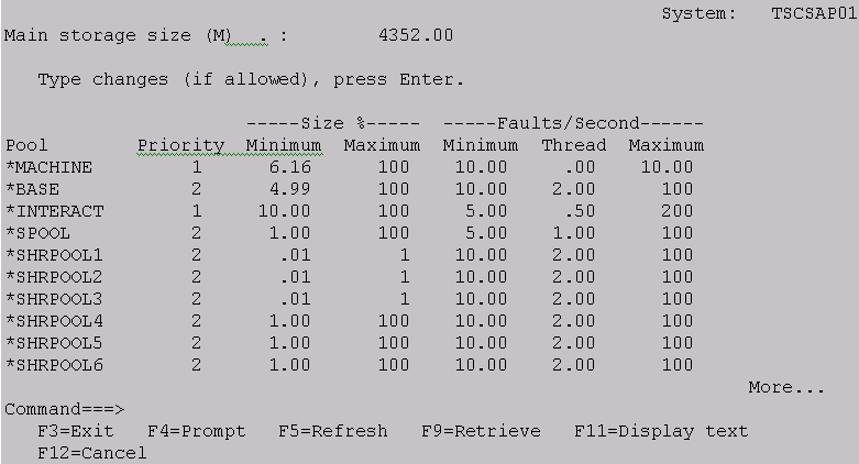
Figure 4: The second WRKSHRPOOL display is used to provide tuning parameters to QPFRADJ.

As you will recall, in the previous article, you separated work into different pools, and I advised you to specify the tuning values for the shared pools that you were using to run your work. Now, I'll tell you what those values mean.

Priority

When the system is shipped, there is no way to know what work is important and what pool it is running in. To adjust the bonus points for a pool, merely change the value of the priority to 1 (high) through 14 (low). By changing the priority of a pool, you can provide some minor direction to the performance adjustment function.

Size %--Maximum and Minimum

The values specified in these two columns control the degree of main storage reassignment performed by the performance adjustment feature.

First, you can specify the minimum amount of memory that you would like allocated to a pool. This can be an important factor for performance in many situations. Here are two examples of situations in which setting the minimum size of the pool will control main storage allocation to one or more pools and provide better system throughput:

1. If jobs in the pool are not getting dispatched because higher-priority work is running, they may lose all of their allocated storage. When they finally get a chance to run, they spend all their time trying to get their information back into main storage. As a result, there will be an increase in I/O operations and faults in the pool. Eventually, the performance adjustment algorithm will recover and rebalance the main storage, but it may take a while, and the jobs will not progress very well.

2. A pool may be dormant for a period of time, and it will lose all its main storage only to return to activity and, once again, require all of the information to be reloaded into main storage. For example, a pool that is used by interactive users who perform a large number of interactions with the system may become dormant when the people entering the transactions leave for lunch. When they return and start entering information, they will experience poor performance until the pool has allocated enough main storage to produce efficient transactions.In both of these instances, you can preserve some of the information that these jobs were using by establishing a reasonable minimum size %.

Now, it's time to look at the maximum size %. The default value for the maximum amount of storage that can be assigned to the shared pools is 100%! That certainly is alarming! Assigning all of main storage to a single pool, even the *MACHINE pool, would certainly cause trouble in all of the other pools in the system. So you need to specify a value other than 100 for each of your shared pools.

Faults/Second--Minimum, Thread, and Maximum

The next three values allow you to specify faulting rates for the pools that are used to run your jobs. The assumptions that have been made for the default values may not reflect the situation in your environment. By modifying these values, you may be able to influence the tuning decisions that are made by the dynamic performance adjustment function.

Once again, Chapter 4 of the iSeries and AS/400 Work Management book provides insight to the origin of the default values and provides methods for you to more properly set the values that are used to assist the QPFRADJ function.

Getting Help from Main Storage Management

So, you now see how you can influence QPFRADJ. You can also use the WRKSHRPOOL command to influence Main Storage Management. In the WRKSHRPOOL display in Figure 3, you see two columns that are called Paging Option.

Paging Option--*FIXED

The default value for the paging option is *FIXED. When this option is in effect, main storage management will use its traditional algorithms. It will retrieve pages only when they are requested, transfer small amounts of information from disk to main storage, and limit the amount of space that is used to cache database pages in memory. This algorithm works fine if there is a shortage of main storage in the pools running the jobs, i.e., the page faults are fairly high. However, since the algorithm was developed when there was much less main storage, you may not be using your main storage effectively.

Paging Option--*CALC

Setting the paging option for a shared pool to *CALC allows Main Storage Management to analyze references to objects in the pool. The analysis is done for each pool that has *CALC specified. As your jobs reference information, one of four reference patterns will be detected. Main Storage Management will use the reference pattern information to make adjustments for certain conditions. There are four types of reference patterns and actions taken by Main Storage Management:

• References are completely random within the objects being used; no adjustments will be made to transfers from disk.
• References are sequential within an object; larger blocks of information will be transferred from disk each time a request is made. In addition, more of the object will be cached in main storage.
• Several references are made to a block of information that is read from disk; larger blocks of information will be transferred from disk for each request.
• Continual references to a portion of an object cause the object to remain in main storage for a lengthy period of time; future requests for information from this type of object will produce large transfers from disk. In addition, if the pages that are being used heavily are being changed, they will be written to disk periodically in order to save their contents in the unlikely event of a system failure.

The entire time that Main Storage Management is making adjustments to the transfers from disk, it continues to monitor the page faulting in the pool. If the page fault rate in the pool begins to get too high (determined by Main Storage Management algorithms), the blocking factors will be reduced. The best part of using *CALC is that all of the analysis is done by the system, so it does not require any work on your part (other than to change the paging option to *CALC). *CALC should be specified for all shared pools.

Because there is such low overhead to provide more efficient Main Storage Management, the paging option should be set to CALC. This is not the default value. Also, when you change to PAGING(*CALC), be sure to specify a the minimum size value on the WRKSHRPOOL display that is much larger than 1!

Removing Troublesome Jobs from Interactive Pools

Occasionally, an interactive job will use an extraordinary amount of main storage. When this happens, other users in the pool can be affected. The system has a function to prevent the storage-intensive jobs from interfering with other users in the pool. I'll use an example to illustrate this function. Consider a classroom (pool) full of students (jobs). While most students are well-behaved and stay within their space (complete their tasks within the timeslice value), there is usually at least one student who will occasionally act up in class (exceed timeslice). Often, these students are not just looking for attention (CPU use), they are pushing other students around (taking more space away from them). Thus, other students in the classroom are disrupted and cannot do their work efficiently. When this occurs, a good teacher (system) will have the student removed from the classroom and sent to the principal's office (another pool). After the student has finished acting up in the principal's office, the student is returned to the classroom to, presumably, behave better (complete the next transaction within the timeslice).

The scenario that I've just described illustrates the function of the QTSEPOOL (Timeslice end pool) system value. This system value can be set to *NONE or *BASE. If the value is *NONE, an interactive job is allowed to stay in the same pool at timeslice end (the student isn't removed from the classroom). If the value is *BASE, the interactive job will be moved from its current pool (classroom) to *BASE (principal's office) in order to finish its work. The QTSEPOOL system value applies only to interactive jobs.

Figures 5 and 6 show the effects of QTSEPOOL.

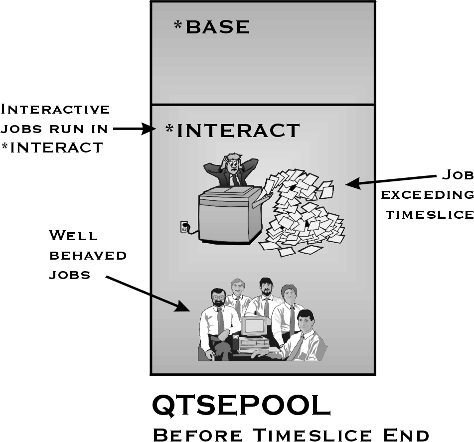
Figure 5: All jobs running in a pool share the same space. Jobs exceeding timeslice often disrupt the contents of the pool.  

Figure 6: The system value QTSEPOOL can be used to move disruptive jobs to *BASE.

By setting the system value to QTSEPOOL, you have removed troublesome jobs from an interactive pool. Troublesome jobs will return to their original pool for any following transactions. The net effect of this function is to provide better performance to more users rather than provide optimum efficiency to storage-intensive operations.

Accessing the System's CPU

Up to now, the only thing that you have been concerned with is the paging and main storage allocations in the pools that your jobs are using. However, another Work Management factor that can affect a job's performance is the Run Priority that it receives when it is initiated by Work Management. To see how this affects a job's performance, it is important to understand how the system schedules jobs to use its CPU.

Dynamic Priority Scheduling

By default, the iSeries uses a dynamic priority scheduling algorithm set by the system value QDYNPTYSCD. While there are a large number of algorithms that can be chosen for dynamic priority scheduling, all of them have the same principals:

1. Distribute the CPU more equitably between the large number and wide variety of jobs running.
2. Recognize the length of time that a job has been waiting for the CPU.
3. Prevent a high-priority job from monopolizing the CPU.

In order to implement these principals on the AS/400, the dynamic priority scheduling implemented an algorithm called Delayed Cost Scheduling.

As the name implies, Delayed Cost Scheduling calculates the cost for the time that a job is in the main storage but has not gained access to the CPU. Since all work in the system is important, costs are calculated for all of the jobs that are running, regardless of their initial priority. When the system is choosing the next job to schedule/dispatch, it uses the job's cost, not its original priority. The chart in Figure 7 provides a schematic view of the dynamic priority scheduling algorithm.

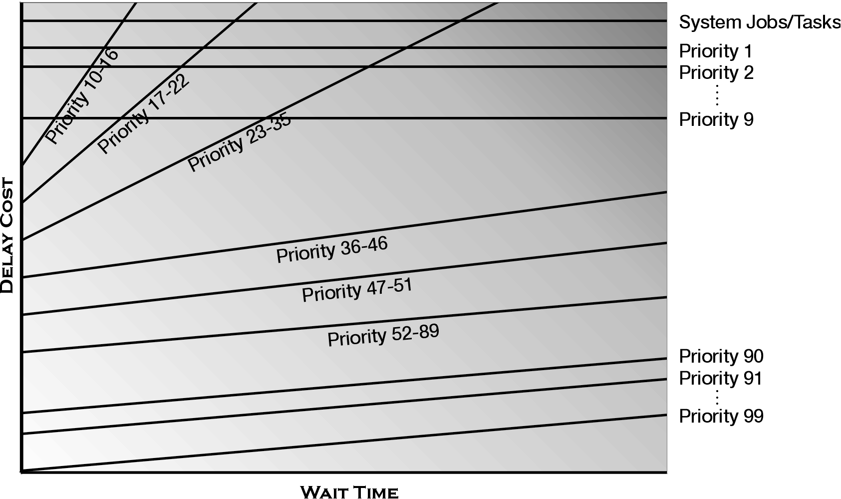
Figure 7: Dynamic priority scheduling uses a delay cost algorithm to determine the scheduling and dispatching of jobs to an available processor.

While this diagram represents the scheduling algorithm very well, it is not easy to understand. It needs a fair amount of explanation in order for you to understand how the system uses the job's RUNPTY value in this scheduling/dispatching scheme. A more complete explanation of Delay Cost Scheduling is given in Chapter 3 of my book. For now, I'll just cover some of the basics. It's also not very easy to see how this scheme provides the benefits that I asserted earlier.

The dynamic priority scheduling algorithm uses the job's run priority as follows:

1. Each job, as it enters the system, has its run priority converted to an initial cost. The job is then placed on the cost curve (line) that is used to determine its wait time costs.

2. At the top of the cost chart, there are some solid flat lines for the system jobs and task and jobs that were assigned a run priority of 1 - 9 when they were initiated. These lines represent fixed priority scheduling. Jobs in these categories will not have any wait time costs added to their original priority. However, they will always be scheduled before any other jobs in the system. Clearly, the system jobs/tasks need to be scheduled before any user jobs are scheduled. Otherwise, the system will not run well. The priority 1 - 9 assignments should be used only for user jobs that are extremely critical--typically, there shouldn't be any.

3. The remainder of the curves on the system represent a range of run priorities. When a job is placed on a cost curve using its initial cost, it is placed on the curve that includes its assigned run priority. That is, a priority 20 job will have a certain initial cost and will be placed on priority 17 - 22 curve; a priority 50 job on the priority 47 - 51 curve, etc.

4. The cost of waiting for a high-priority job is higher than the cost for a low-priority job. This is represented by the slope of each of the cost lines. The curves that are used for jobs with higher run priorities have a steeper slope than the curves used for jobs with lower run priorities.

5. Finally, notice that the cost of a job can exceed the cost of the system job/tasks and the priority 1 - 9 jobs (represented by the dashed line). Although the cost of these jobs may be higher, they will not be dispatched before the system jobs/tasks or the priority 1 - 9 jobs.

6. The cost curve priority ranges are designed to separate jobs that use the typical (default) run priority values. Thus the system console and spool writers are on one curve, interactive jobs on another, and batch jobs on yet another. This helps to preserve the importance of the run priority that you assigned to the jobs.

So, using these basic cost calculations, you can now see that a batch job running on the priority 50 curve will eventually increase in cost until its cost is higher than a newly arrived priority 20 job. Notice, however, that jobs on the run priority 20 curve will increase in cost faster than the customers on the run priority 50 cost curve. They have a higher cost of waiting. It will not be long before the new arrival on the run priority cost curve will be scheduled to use the CPU. That's the purpose of delay cost: allow lower-priority, but still important, jobs an opportunity to use the processor when they have waited a long time (their cost has increased) while limiting the wait time for higher priority jobs by assigning a higher cost to the wait time.

Providing Special Run-Time Attributes

Now that you have separated your important front-desk users, have you done enough? In many instances, yes. In many others, no. While separating the jobs helps them keep their pages in main storage, they must still compete for disk and processor resources. You can influence a job's ability to utilize these resources more efficiently with the run-time attributes that you assign to a job when it is started by the subsystem. There are three main run-time attributes: PURGE, TIMESLICE, and RUNPTY. In order to help your special jobs, you may need to adjust these values. But which values should you adjust, and what values should you use

Let's review the purposes of these run time attributes:

1. PURGE--The PURGE run-time attribute instructs the system how to manage the pages in main storage that are unique to each job and are contained in the Process Access Group (PAG). By altering the PURGE attribute, you may be able to reduce disk operations and reduce the disk component of the front desk's response. Unfortunately, with the demise of the PAG, modifying this attribute is of little use.

2. TIMESLICE--The TIMESLICE value is used to limit the amount of CPU time that a job can use during any single transaction. For your front desk jobs, there should be few if any transactions that will use 2 seconds of CPU time (the default for TIMESLICE). Unless your most important jobs average more than 1 second of CPU time per transaction, changing this value will be of little benefit. In fact, most environments will see no improvement.

3. RUNPTY--The RUNPTY value is used to establish the initial cost of a job whenever it enters a transaction to be processed. In addition, RUNPTY determines which of your delay cost curves will be used to calculate the increase in cost as your jobs wait for resources. Eventually, you reach a run-time value that will provide additional benefits to your interactive job.

You have now identified which attribute to change, but what should the setting should be? Go back and look at the delay cost curves, as shown in Figure 8.

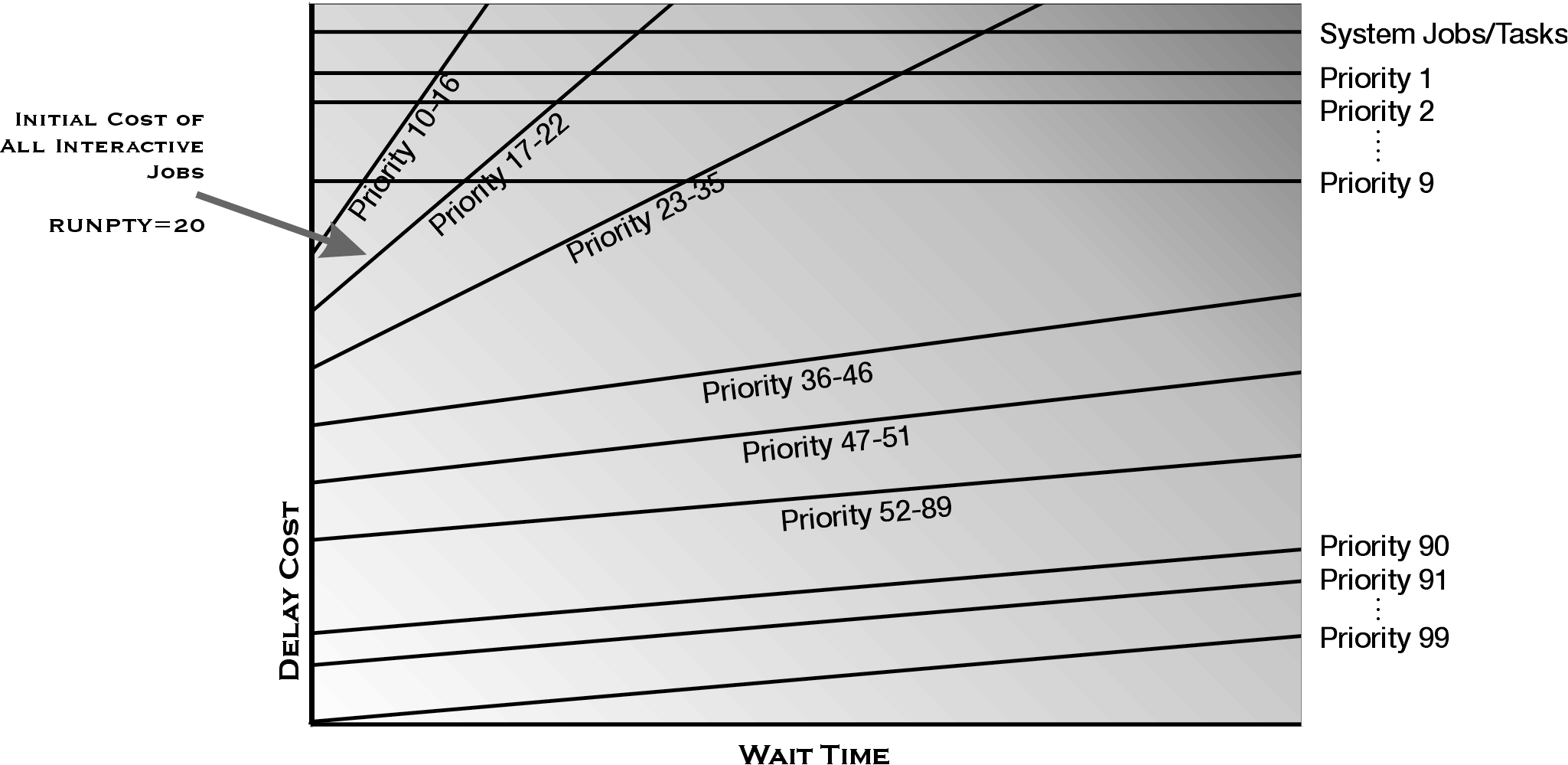
Figure 8: This diagram shows the system delay cost curves used to schedule and dispatch work in your system.

The RUNPTY value is found in the class that is named in the routing entry that is used when the job is started. Since all of your interactive routing entries specify QINTER as the class (CLS), all the jobs are assigned the same run-time attributes. So, since all of your routing entries are using the QINTER class, you can't just change the class. Otherwise, everybody will pick up the same run-time attributes again. You need to create a new class that has a RUNPTY value that is different from the value in the QINTER class (20). You also need to change the routing entry at SEQNBR(12) to use the new class (Figure 9). All you need to do is figure out the value of RUNPTY in your new class.

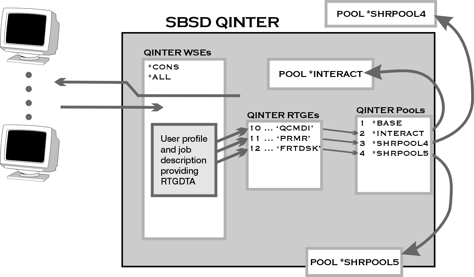
Figure 9: The QINTER routing entry with sequence number 12 is changed to use a different class than the routing entries at sequence numbers 10 and 11.

Look at the delay cost diagram in Figure 8. If you change the RUNPTY for your valuable users to 19, 18, or 17, you'll still be on the same cost curve as all of the other interactive jobs. That will help some. But notice what would happen if you changed the RUNPTY of your users to 16. You will have placed your users on a different cost curve. In addition, the cost of waiting increases faster (the slope of the line is steeper) on the RUNPTY 16 curve. In addition, there is no CPU usage penalty on the RUNPTY 16 cost curve. That is, the important jobs will not be reassigned to a lower cost curve regardless of the amount of the CPU that they use. Sounds like you ought to set the RUNPTY to 16, doesn't it?

Run these commands:

You can take the default values for all of the other parameters of the Create Class (CRTCLS) command. And you're done! Well, almost. The run-time attributes are assigned at the time a job is started. In order to have interactive jobs reassigned to different pools or to be given different run-time attributes, users will need to sign off their workstations and sign on again. But, as long as it means preferential treatment, most users will be willing to perform that simple task.

Well, I have once again covered a lot of information, which is also included in Chapters 3 and 4 of iSeries and AS/400 Work Management. The information in these two articles should provide you with techniques to improve performance in your environment. In the final article in this series, I will look at information that is not in the current edition of the book. My focus will be on Independent Auxiliary Storage Pools (IASPs). This new iSeries technology requires Work Management assistance in order to access information stored in an Auxiliary Storage Pool (ASP).

Chuck Stupca is a Senior Programmer in the IBM iSeries Technology Center in Rochester, Minnesota, where he is responsible for performance, clustering, and Independent ASP education and consulting. He can be reached via email at This email address is being protected from spambots. You need JavaScript enabled to view it..

Also Read

TD/OMS and Gravity “Milestone 1” Enhancements Streamline Efficiency and Advance Application Development Potential for Re...

Now Let’s Consider Vendor Maintenance

Know Where Your Maintenance Stands