Next in our series on Artificial Intelligence fundamentals, we take a look at different types of Machine Learning methods.  If you missed them, Read Part 1, Understanding Data, Part 2: Artificial Intelligence, Machine Learning, and Deep Learning, and Part 3: Data Preparation and Model Tuning here.

By Roger Sanders

The illustration shown in Figure 1 provides an overview of the different types of machine learning (ML) methods that are available, along with examples of where each method might be used. The most common types of learning methods utilized are supervised learning and unsupervised learning.

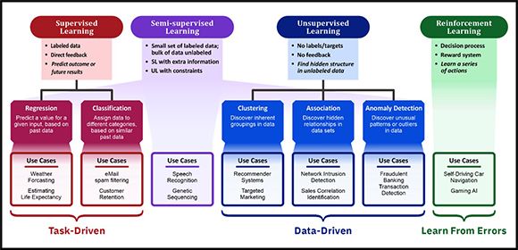
Figure 1: Machine learning methods

 Supervised learning typically begins with an established set of data and a certain understanding of how that data is classified. In other words, a model is trained with a fully labeled data set, fully labeled meaning that each example in the training data set is tagged with the answer the model should be able to come up with on its own. Supervised learning methods are further categorized as being regression or classification in nature.

Regression models are used to help understand the correlation between data variables. For instance, a weather forecasting model will typically use some form of regression analysis to apply known historical weather patterns to current weather conditions to make a weather prediction. Classification models, on the other hand, produce output that identifies input data as being a member of a particular class or group. For example, if you have a training data set that contains hundreds of images of flowers, along with a description of the flower in each image, a trained classification model should be able to correctly classify the flower in an image it has never seen before.

With unsupervised learning, a model is given an unlabeled data set without explicit instructions on what to do with it. The model then attempts to make sense of the data by extracting useful features and patterns on its own. Depending on the problem at hand, an unsupervised learning model can extract patterns in one of three ways:

• Clustering: Without being an expert entomologist, it’s possible to look at a collection of insects and separate them roughly by species, relying on cues like color, size, and shape. That’s how models that use clustering work: they look for data that is similar to other data and group this data together.
• Association: Fill an online shopping cart with shampoo and conditioner and an e-commerce web site may recommend that you add soap or a hairbrush to your order. This is an example of association – certain features of a data sample correlate with other features and by looking at key attributes of a data point, an association learning model can identify other attributes they’re frequently associated with.
• Anomaly detection: Anomaly detection models look for unusual patterns or outliers in a data set. For instance, if the same credit card number is used to make a purchase in Raleigh, North Carolina and Lisbon, Portugal within a four-hour window, that’s cause for suspicion. If the credit card owner lives in Raleigh, a bank using an anomaly detection model would probably flag or block the purchase in Lisbon, treating it as a fraudulent transaction. (Which is why many banks ask that you notify them ahead of time before you travel outside your country of residence if you plan on using their card.)

Semi-supervised learning is, for the most part, a method for training models with a data set that consists of a small amount of labeled and a much larger amount of unlabeled data. This learning method is particularly useful when extracting relevant features from data is difficult and labeling all the data available is too costly or time intensive. Examples of where semi-supervised learning might be used include speech recognition and genetic sequencing.

Finally, reinforcement learning is a behavioral learning method. This type of learning differs greatly from the other learning methods because a model isn’t trained with a sample data set. Instead, it learns, through trial and error, the optimal way to attain a particular goal or solve the problem at hand. Thus, a sequence of successful decisions will result in a model’s process being “reinforced.” To make its choices, a reinforcement learning model relies on learnings from prior feedback, as well as exploration of new tactics. It’s an iterative process and the more feedback the model receives, the better it becomes. Reinforcement learning is the training method that’s used to learn and play popular video games. It’s also the method being used to create autonomous (self-driving) vehicles.

Regression

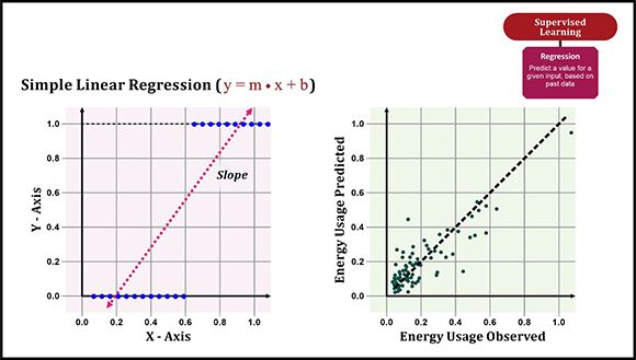
Figure 2: An example of simple linear regression

As mentioned earlier, regression is a form of supervised learning that is used to help understand the correlation between data variables. Mathematically, regression is a statistical way to establish a relationship between a dependent variable and one or more independent variables. For example, if we say that Age = 5 * Height + Weight, we are establishing a relationship between the height and weight of a person with his or her age. Regression is used primarily for forecasting and to identify cause and effect relationships.

There are a variety of regression techniques available, and each has its own use case where it is best suited. However, linear regression is perhaps one of the most well known and most understood algorithms used in statistics and ML today. Therefore, it is often the first algorithm a data scientist learns (and turns to for problem solving).

Simple linear regression uses the mathematical equation y = m * x + b to model data in a traditional slope-intercept form:

• m and b represent the variables the model will attempt to “learn” from so it can produce the most accurate results
• x represents the model’s input data
• y represents the model’s output or prediction

A simple linear regression model is trained by examining as many data pairs (x, y) as possible, and calculating the position and slope of a line that minimizes the total distance between the data points used and the line itself. In other words, by calculating the slope (m) and y-intercept (b) for a line that best approximates observations seen in the data. The example plot shown on the right-hand side of Figure 2 illustrates how simple linear regression might be used to predict energy consumption for a set of buildings.

Regression techniques run the gamut from simple (linear regression) to complex (regularized linear regression, polynomial regression, multi-variable linear regression, decision trees, random forest regressions, and neural networks, among others). And a more complex linear equation might be used if more than one independent variable is required, if the type or number of dependent variables used changes, or if the shape of the regression line is something other than a traditional slope-y-intercept.

Going back to the example of using regression to predict the energy consumption (in kWh) of a set of buildings, if you wanted to further refine the model used by gathering information such as the age of each building, the number of floors in each building, the inhabited square footage of each floor, and the number of electrical outlets available, you might decide to use multi-variable linear regression because of the different input factors (building age, number of floors, square footage, etc.) utilized. The principle is the same as with simple linear regression, but in this case the “y-intercept line” created occurs in a multi-dimensional space, based on the number of variables used. Once a model using this type of regression is properly trained, if you have access to the characteristics of a different building (it’s age, number of floors, square footage, etc.) but you don’t know what its energy consumption looks like, you can use the fitted line to approximate this value.

It’s important to note that linear regression can also be used to estimate the weight of each factor that contributes to the final prediction. So, for example, once a formula for predicting building energy consumption has been created, it’s possible to determine whether building age, number of floors, square footage, or outlet usage is the most important factor to take into consideration when making these types of predictions.

Classification (logistic regression)

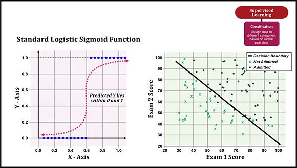
Figure 3: Classification using logistic regression

As we saw earlier, classification models produce output that identifies input data as being a member of a particular class or group. And an algorithm that is frequently used for classification models is logistic regression, which gets its name from the function that serves as its core – the logistic function (also known as the Sigmoid function). This function was developed in the late 1840’s to model the exponential growth of an area’s population, taking carrying capacity into account. (The carrying capacity of an ecosystem is the maximum population size that can be supported indefinitely, given the resources and services available within that ecosystem. A simple example is the number of people who could survive in a lifeboat, which depends largely on how much food and water is available, how much each person must eat and drink every day to stay alive, and how many days everyone must remain in the lifeboat before they are rescued.)

Mathematically, logistic regression measures the relationship between a categorical dependent variable and one or more independent variables by estimating probabilities. (The term binary regression implies only one independent variable is used; the term multinomial regression implies multiple independent variables are used.) The logistic function itself produces an S-shaped curve that can be used to map any real-valued number to a value between 0 and 1. The resulting number is a probability score which, in the case of logistic regression, reflects the likelihood that something belongs to a particular group or class. You can think of logistic regression as a kind of “on-off switch” where input can build for a long time while still being interpreted as “off” (0), but that at some point, flips to “on” (1) and remains there forever. A threshold is used to indicate at what value the switch flips from “off” to “on” and often, this value is 0.5, meaning that if the output of the logistic function is more than 0.5, the outcome is classified as being 1 or TRUE, and if it is less than 0.5, it is classified as being 0 or FALSE. (A probability score close to 1 means the observation is very likely to be part of a particular group or class.)

As an example, consider a logistic regression model that is used to determine whether a student will be admitted to a prestigious university. If the model infers a value of 0.932, based solely on the scores of two admission exams, it implies that there is a 93.2% probability that a student will be admitted (assuming there is no limit to the number of students allowed and the threshold used is 0.5). More precisely, the set of students for which the model predicts 0.932 will be admitted 93.2% of the time; 6.8% of the time they will not. The plot shown on the right-hand side of Figure 3 illustrates how logistic regression might be used to draw a line that represents what the admission decision boundary looks like, based on historical test scores and admittance selection information.

Because logistic regression is a linear algorithm, it can be a good place to start when a simple classification model is needed. Models built using this algorithm are incredibly easy to implement and are very efficient to train. They don’t require a lot of computational resources, don’t require input features to be scaled, don’t require tuning, are highly interpretable, and produce well-calibrated, predicted probabilities. However, logistic regression models work better when attributes that are unrelated to the output variable or that are very similar to each other (correlated) are removed. So, feature engineering and dimensionality reduction plays an important part in how well a logistic regression model performs.

One disadvantage with logistic regression is that it cannot be used to solve non-linear problems. Since its output is discrete, it can only predict a categorical outcome. It is also vulnerable to overfitting. So, it’s not one of the most powerful classification algorithms available and can easily be outperformed by other, nonlinear classifiers such as decision trees, random forests, support vector machines (SVMs), and neural networks. Another disadvantage is that it is only useful if all the important independent variables have been identified. That said, logistic regression models do well in many tasks. Not only does logistic regression aid in classification, but it also provides probabilities, which can be an advantage over models that only provide final classifications. Sometimes, knowing that an instance has a 99% probability of being part of a particular group or class, compared to having a 51% probability can make a big difference.

Clustering

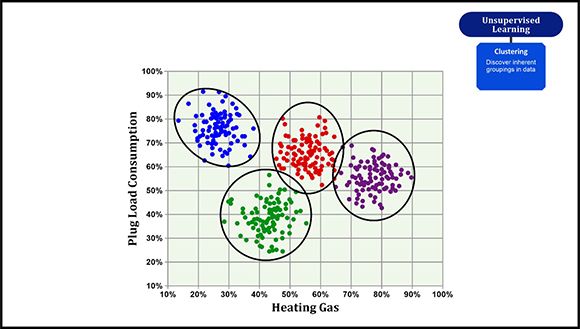
Figure 4: Example of clustering

So far, we have only explored supervised machine learning (ML), which typically begins with an established set of data and an understanding of how that data is classified. Thus, supervised learning models are trained with data that has already been tagged with the answers models are expected to come up with on their own. However, data does not always come with predefined labels. And this is where unsupervised machine learning comes into play.

Unsupervised ML algorithms infer patterns from a data set without reference to known, or labeled, outcomes. Because there is no way to know in advance what the values for the output data might be, unsupervised learning methods cannot be directly applied to regression or classification problems. Instead, this type of learning is often used to find meaningful structure, underlying processes, generative features, and groupings that are inherent in a data set.

The most common unsupervised learning method used is cluster analysis (or clustering), which relies on some measure of similarity to find hidden patterns or groupings in data. (In statistics, a similarity measure is a function that quantifies the similarity between two objects.) In theory, data points placed in the same group should have similar properties or features, while data points placed in different groups should have highly dissimilar characteristics. But in reality, the similarity between groups can be overestimated because some assumptions must be made about what constitutes the sameness of data points.

Some of the more common clustering algorithms used include:

• K-Means clustering: Data is partitioned into a fixed number (k) of distinct clusters (groups of data points that have similar features) based on distance to the real or imaginary point at the center of a cluster (otherwise known as the centroid). The K-Means algorithm starts by randomly defining k centroids and assigning each data point to the closest centroid, based on the straight-line distance between the data point and the centroid. Then, it goes through each centroid and calculates the mean (average) of all points belonging to the centroid, and the mean value becomes the new centroid. This process is repeated until there is no change in centroid values, or until a previously determined number of iterations have been performed. (This number is provided via a model hyperparameter.) At this point it is assumed that the data points have been accurately grouped.
• Hierarchical clustering: Clusters formed with this method result in a tree-type structure based on hierarchy – new clusters are created using the cluster previously formed. There are two approaches to this method of clustering: agglomerative (a “bottom-up” approach) and divisive (a “top-down” approach). With the agglomerative method, each observation starts in its own cluster, and pairs of clusters are merged as one moves up the hierarchy; with the divisive method, all observations start in a single cluster, and splits are performed recursively as one moves down the hierarchy.
• Density-Based Spatial Clustering of Applications with Noise (DBSCAN): Clusters are formed by seeking areas in the data that have a high density of observations (“clusters”), versus areas of the data that are not very dense (“noise”). The idea is that if a particular point belongs to a cluster, it should be near lots of other points in that cluster. To use DBSCAN, we must first define two parameters: a positive number representing distance (epsilon) and a natural number specifying the minimum number of points allowed in a cluster (minpoints). DBSCAN then picks an arbitrary point in the data set and if there are more than minpoints points within a distance of epsilon from that point, (including the original point itself), all of these points are assumed to be part of a "cluster". Then, all the new points are checked to see if they too have more than minpoints points within a distance of epsilon, growing the cluster recursively, if so. Eventually, when no more points can be added, a new point is arbitrarily chosen, and the process is repeated. If a point that has fewer than minPoints points in its epsilon ball is chosen and that point is not part of any other cluster, it's considered point of a "noise”.
• Mean-Shift clustering: Clusters are formed by assigning data points to clusters iteratively, and then shifting points towards the highest density of data points within the region. Mean-Shift works by fixing a window (or radius) around each data point, computing the mean (average) of all data within that window, and then shifting the window to the mean and repeating the process until all cluster centroids available have been defined. Data points in the windows around the centroids are then filtered in a post-processing stage to eliminate near-duplicates, forming the final set of center points and their corresponding groups. Unlike K-Means clustering, mean-shift clustering does not have to be told the number of clusters to look for in advance. Instead, the number of clusters available is determined by the data.
• Gaussian mixture models (GMMs): GMMs attempt to find a mixture of multi-dimensional Gaussian probability distributions that best model an input data set – with GMMs it is assumed that the data points are Gaussian distributed, which is a less restrictive assumption than saying they are circular by using the mean. (Gaussian Distributions have a bell-shaped curve, with the data points symmetrically distributed around the mean value.) In the simplest case, GMM can be used to find clusters in the same manner as K-Means. But, because GMM contains a probabilistic model for representing normally distributed sub-populations within an overall population, it can also provide probabilities that a given data point belongs to each of the clusters possible. The result is that each cluster is not associated with a hard-edged sphere, but with a smooth Gaussian model. Although GMM is often categorized as a clustering algorithm, fundamentally it is an algorithm that is designed for density estimation.

It’s not important that you understand exactly how the clustering algorithms presented here work – that falls under the domain of a data scientist. However, it is good to be familiar with the names of some of the more common algorithms used.

Association

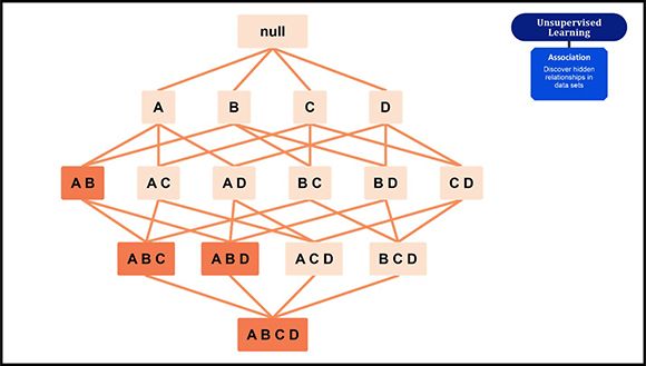
Figure 5: Association

Association is an unsupervised learning technique that is used to identify hidden correlations in data by applying some measure of “interestingness” to generate an association rule for new searches. Association rule algorithms count the frequency of complimentary occurrences, or associations, across a large collection of items or actions. The goal is to find associations that take place together far more often than you would find in a random sampling of possibilities. This rule-based approach is a fast and powerful tool for mining categorized, non-numeric databases. Typical applications include market-basket data analysis, web usage data mining, cross-marketing, loss-leader analysis, continuous production, and the analysis of genomic data.

Association learning relies on the concept of If-Then statements, such as “If A then B”. The If element (A) is called the antecedent and the Then element (B) is known as a consequent. Some association or relation between two items is known as single cardinality and as the number of items increases, cardinality increases accordingly.

To illustrate how association rules are found, let’s look at a simple supermarket market-basket analysis. Walk into any supermarket and you will find products that are often purchased together located on the same shelf or aisle (or somewhere close by). To identify frequently bought items and determine whether they are normally purchased together, an association rule makes use of some, if not all of the following metrics:

• Support – How frequently an item appears in the dataset. (Which items are bought more frequently than others?)
• Confidence – How often items A and B occur together in the dataset when the occurrence of A is already given. (How confident are we that one item (B) will be purchased, given that another item (A) has already been purchased?)
• Lift – A measure that indicates whether the probability of buying one item (B) increases or decreases given the purchase of a different item (A). Lift has three possible values:
  • 1: The probability of occurrence of antecedent and consequent is independent of each other.
  • > 1: The degree to which the two items are dependent to each other.
  • < 1: One item is a substitute for other items, which means that one item has a negative effect on another.
• Conviction – A measure that compares the probability that one item (A) is purchased without another (B) with the actual frequency of the appearance of one item (A) without the other (B). In contrast to lift, conviction is a directed measure and is used to evaluate the directional relationship between items.

Association rule learning is typically performed using one of three distinct algorithms:

• Apriori algorithm: Used to calculate the association rules between objects; that is, how two or more objects are related to one another. This algorithm proceeds by identifying the frequent individual items in a transactional database and extending them to larger and larger item sets so long as those item sets appear sufficiently often in the database. It uses a breadth-first search and Hash Tree to calculate the item set efficiently.

The Apriori algorithm is used primarily for market-basket analysis to understand which products are frequently bought together. It can also be used in the healthcare field to find drug reactions for patients.

• Eclat (Equivalence Class Transformation) algorithm: This algorithm uses a depth-first search technique to find frequent item sets in a transactional database. Unlike the Apriori algorithm, which is designed to work with horizontal data sets, the Eclat algorithm is applicable only with vertical data sets. The Eclat algorithm also scans the database once, whereas the Apriori algorithm scans the original database repeatedly. This enables the Eclat algorithm to execute much faster than the Apriori algorithm. However, this algorithm does not provide Confidence and Lift metrics. Thus, users must make a choice between speed of execution and utilizing more metrics.

When dealing with a larger dataset, the Apriori algorithm tends to shine; the Eclat algorithm, on the other hand, works better with small and medium datasets.

• F-P (Frequent Pattern) Growth algorithm: This algorithm is essentially an improved version of the Apriori Algorithm – it only scans the original database twice and uses a tree structure (FP-tree) to store information. The root of the tree represents null, each node represents an item, and the association of the nodes form the item sets. (Order is maintained as the tree is formed.) Once an FP-tree has been constructed, it uses a recursive “divide-and-conquer” approach to mine for frequent item sets.

Anomaly detection

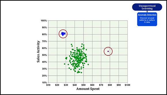
Figure 6: Anomaly detection

Anomaly detection (also known as outlier detection) refers to the process of identifying rare items, events, or observations that raise suspicions by differing significantly from the bulk of the data. Common applications of anomaly detection include fraud detection in financial transactions, equipment malfunction, identification of structural defects, fault detection, and predictive maintenance.

Usually, there are three types of anomalies/outliers data scientists encounter:

• Global outliers – When a data point has a value that is far outside all the other data point value ranges in a dataset. In other words, a rare event. For example, if you have an average American salary added to your bank account every month, but one day receive a million dollars, that will appear as a global anomaly to the bank’s analytics team.
• Contextual outliers – When a data point has a value that doesn’t correspond with what is expected for a similar data point in the same context. For example, it’s normal for retailers to experience an increase in customer traffic during the holiday season. However, if a sudden boost happens outside a holiday or sales event, that indicates a contextual outlier.
• Collective outliers – When a subset of data points deviate from the normal behavior. In general, tech companies tend to grow bigger and bigger. Some companies may shrink, but that’s not a general trend. However, if many companies suddenly show a decrease in revenue during the same period of time, that would be indicative of a collective outlier.

ML algorithms frequently used for anomaly detection (depending on the dataset size and the type of the problem) include:

• Local outlier factor (LOF): Probably the most common technique for anomaly detection, this algorithm computes the local density deviation of a given data point with respect to its neighboring data points. If a data point has a lower density than its neighbors, it is considered an outlier.
• K-nearest neighbors (KNN): While KNN is an algorithm that is often used for classification, when it is applied to anomaly detection problems, it can be a useful tool because it enables users to easily visualize data points on a scatterplot and make anomaly detection much more intuitive. Another benefit of KNN is that it works well with both small and large datasets.

Instead of learning ‘normal’ and ‘abnormal’ values to solve a classification problem, KNN doesn’t perform any actual learning. Instead, a data scientist defines a range of normal and abnormal values manually, and the algorithm breaks this representation into classes, by itself.

• Support Vector Machine (SVM): SVM is also an algorithm that is often used for classification. This algorithm uses hyperplanes in multi-dimensional space to divide data points into classes. (SVM is usually applied when there are more than one classes involved in the problem.) However, in anomaly detection it’s also used for single class problems. The model is trained to learn the ‘norm’ and can identify whether unfamiliar data belongs to this class or represents an anomaly.
• DBSCAN: Based on the principle of density, DBSCAN can uncover clusters in large spatial datasets by looking at the local density of the data points and generally shows good results when used for anomaly detection. The points that do not belong to any cluster get their own class (-1) so they are easy to identify. This algorithm handles outliers well when the data is represented by non-discrete data points.
• Autoencoders: Autoencoders are a specific type of feed-forward neural networks where the input is the same as the output. They compress the input into a lower-dimensional code and then reconstruct the output from this representation. (The code is a compact “summary” or “compression” of the input.) When trying to reconstruct the original data from its compact representation, the reconstruction may not resemble the original data, thus helping to detect anomalies when they occur.
• Bayesian networks: A Bayesian network is a representation of a joint probability distribution of a set of random variables with a possible mutual causal relationship. The network consists of nodes representing the random variables, edges between pairs of nodes representing the causal relationship of these nodes, and a conditional probability distribution in each of the nodes. Bayesian networks are ideal for examining an event that occurred and predicting the likelihood that any one of several possible known causes was the contributing factor.

Bayesian networks can be used to discover anomalies even in high-dimensional data. This method is used when the anomalies being searched for are more subtle and harder to discover and visualizing them on a plot might not produce the desired results.

Ensemble methods

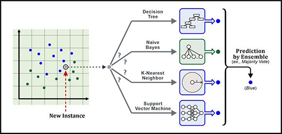
Figure 7: Ensemble methods

Ensemble methods are meta-algorithms that are used to combine several machine learning (ML) techniques to create a single predictive model. The main principle behind ensemble modelling is to group several weaker models together to form a single strong model that can make more accurate predictions. Most of the errors that occur in ML are due to noise, bias, and variance. So, ensemble methods help to minimize these factors.

Ensemble methods can be divided into two groups: sequential ensemble methods where base ML learners are generated sequentially and parallel ensemble methods where base learners are generated in parallel. (In ML, learners are programs or algorithms that are used to train an ML model.) The basic motivation behind sequential ensemble methods is to exploit the dependence between the base learners used – overall performance can be boosted by assigning previously mislabeled examples higher weights. On the other hand, the motivation behind parallel ensemble methods is to exploit independence between the base learners used since error can be reduced dramatically by averaging. A popular sequential ensemble method is AdaBoost (short for “Adaptive Boosting”), which is a successful boosting algorithm that was developed for binary classification. A popular parallel ensemble method is Random Forest, which is one of the most widely used algorithms for feature selection.

Most ensemble methods use a single base learning algorithm to produce homogeneous base learners. In other words, learners of the same type. The result is known as homogeneous ensembles. However, there are some methods that use heterogeneous learners – that is, learners of different types – to create heterogeneous ensembles. For an ensemble method to be more accurate than any of its individual members, the base learners used must be as accurate and diverse as possible.

Three ensemble techniques that are often used to decrease variance, reduce bias, and improve predictions are bagging, boosting, and stacking. Bagging stands for Bootstrap Aggregating and it works by creating random sample subsets of training data from the full training data set provided, and then building a model (classifier or decision tree) for every sample subset. The results of these multiple models are then combined using averaging or majority voting. Because each model is exposed to a different subset of data and their collective output is gathered at the end, overfitting is avoided. Thus, bagging helps to reduce variance error. (Random Forest actually uses this concept but goes one step further to reduce variance by randomly choosing a subset of features for each bootstrapped sample to make the data splits while training.)

Boosting is a sequential technique in which the first algorithm is trained on the entire data set and subsequent algorithms are built by fitting the residuals of the first algorithm, thus giving higher weight to those observations that were poorly predicted by the previous model. If an observation was classified incorrectly, its weight is increased or decreased, as appropriate. Boosting relies on creating a series of weak learners, each of which might not be good for the data set as a whole but is great for some portion of it. Thus, each model actually boosts the performance of the ensemble. Boosting in general decreases bias error and builds strong predictive models. However, it also can lead to overfitting. Because of this, parameter tuning is crucial when boosting algorithms are used.

Stacking is an ensemble learning technique that combines multiple classification or regression models using a meta-classifier or meta-regressor. The base level models are trained on a complete training data set, then the meta-model is trained on the outputs of the base level model, as features. The base level often consists of different learning algorithms; therefore, stacking ensembles are often heterogeneous in nature. Stacking is used primarily to improve predictions.

Stay Tuned

In the next part of this article series, we’ll look at deep learning and the workhorse of deep learning: neural networks.

Roger E. Sanders is a Principal Sales Enablement & Skills Content Specialist at IBM. He has worked with Db2 (formerly DB2 for Linux, UNIX, and Windows) since it was first introduced on the IBM PC (1991) and is the author of 26 books on relational database technology (25 on Db2; one on ODBC). For 10 years he authored the “Distributed DBA” column in IBM Data Magazine, and he has written articles for publications like Certification Magazine, Database Trends and Applications, and IDUG Solutions Journal (the official magazine of the International Db2 User's Group), as well as tutorials and articles for IBM's developerWorks website. In 2019, he edited the manuscript and prepared illustrations for the book “Artificial Intelligence, Evolution and Revolution” by Steven Astorino, Mark Simmonds, and Dr. Jean-Francois Puget.

From 2008 to 2015, Roger was recognized as an IBM Champion for his contributions to the IBM Data Management community; in 2012 he was recognized as an IBM developerWorks Master Author, Level 2 (for his contributions to the IBM developerWorks community); and, in 2021 he was recognized as an IBM Redbooks Platinum Author. He lives in Fuquay Varina, North Carolina.

---

MC Press books written by Roger E. Sanders available now on the MC Press Bookstore.

		QuickStart Guide to Db2 Development with Python Discover how Python, SQL, and Db2 can successfully be used with each other. List Price $9.95 Now On Sale
		DB2 10.5 Fundamentals for LUW (Exam 615) Don't even think about attempting to take the DB2 Fundamentals exam without this indispensable study guide. List Price $79.95 Now On Sale
		DB2 10.1 Fundamentals (Exam 610) Let one of the world's leading DB2 authors and a participant in the exam development help you succeed. List Price $79.95 Now On Sale
		Artificial Intelligence: Evolution and Revolution Operational AI has become available to the masses, setting the wheels in motion for a worldwide AI revolution that has never been seen before. List Price $16.95 Now On Sale
		DB2 10.5 DBA for LUW Upgrade from DB2 10.1: Certification Study Notes Here's everything you need to know to take and pass Exam 311, complete with a practice exam and study key. List Price $21.95 Now On Sale
		From Idea to Print Here's everything you need to know to turn your technical knowledge and expertise into a published article or book. List Price $49.95 Now On Sale
		DB2 9 Fundamentals (Exam 730) Use this review before taking the test to prove you've mastered the basics of DB2 9. List Price $59.95 Now On Sale
		DB2 9 for Linux, UNIX, and Windows Database Administration (Exam 731) Use this indispensable study guide to prepare to take, and pass, Exam 731. List Price $64.95 Now On Sale
		DB2 9.7 for Linux, UNIX, and Windows Database Administration (Exam 541) Get ready to take the DB2 9.7 certification exam with this handy study guide. List Price $21.95 Now On Sale
		DB2 9 for Linux, UNIX, and Windows Advanced Database Administration (Exam 734) Review all exam topics and take the included practice test to be sure you're ready on testing day. List Price $64.95 Now On Sale
		DB2 9 for Linux, UNIX, and Windows Database Administration Upgrade (Exam 736) Prep for success with the master of DB2 certification study guides! List Price $34.95 Now On Sale
		Data Fabric: An Intelligent Data Architecture for AI This book explains the concepts and values that a data fabric approach can deliver to both technical and business communities. List Price $19.95 Now On Sale

Also Read

How AI Will Stoke Rather Than Dampen Job Markets

Putting the Brakes on the AI “Runaway Train” Myth

Artificial Intelligence, Part 6: Measuring Quality and Understanding Challenges